An inverse gradient between socioeconomic status (SES) and mortality in Western countries has been solidly established.¹ This gradient is well documented for all-cause mortality as well as for some specific causes of death, including cardiovascular diseases^2–4 and several cancers.^4–6 Although most pronounced during middle age, it is also observed among the elderly.⁷

The prevalence of numerous risk factors for potentially fatal diseases (again, cardiovascular diseases and cancers) also tends to be inversely associated with SES. Compared with populations with high SES, less advantaged populations tend to smoke more⁸ and to eat less fresh fruit and vegetables⁹ and more saturated fat.¹⁰ They also face more types of psychosocial stress (eg, financial strain, job insecurity, low control at work)¹¹ and receive poorer healthcare (accessibility, use, quality of care).¹² Nonetheless, it remains difficult to quantify the extent to which the unequal distribution of these risk factors in populations with divergent SES explains these socioeconomic mortality gradients.

Moreover, relatively few studies have examined the contribution of environmental exposures, such as air pollution, to socioeconomic health inequalities.¹³ Several authors hypothesise that air pollution contributes to creating or accentuating the socioeconomic disparities seen in various diseases (including cancer,¹⁴ asthma¹⁵ and cardiovascular diseases¹⁶) and thus in premature death rates.¹⁷ Two types of potential mechanisms have been suggested.

• Firstly, populations with low SES may be more frequently or more intensely exposed to air pollution than those with high SES.^18,19 Nonetheless, Bowen concluded in 2002 that the results of studies documenting the distribution of exposure to air pollution in populations with different SES remain “mixed and inconclusive”.²⁰ Later studies^21–24 support this observation. The methodological diversity of these studies and the variety of their settings²² may partly explain the heterogeneity of their results.

• Secondly, populations with low SES may be more susceptible to air pollution than those with high SES¹⁸ in that several factors which are more prevalent in less advantaged populations may be effect modifiers of the relationship between pollution and mortality. These include poor health status (for example, diabetes, obesity and chronic obstructive pulmonary disease),¹⁸ addictions (including smoking)²⁵ and multiple pollutant exposures (passive smoking, occupational exposure) likely to act in addition to or in synergy with urban pollution,²⁵ and difficulties with access to healthcare.^19,26 Less obvious factors, such as psychosocial stress,^17,19,26 low intake of proteins, vitamins and minerals,¹⁹ and even genetic make-up¹⁷ may also play a part.

This review examines studies that tested this second hypothesis about mortality, by asking if SES is a sensitivity factor in the relationship between atmospheric pollution and mortality.

METHODS

We searched Medline from its inception to the end of April 2006, using three-MeSH term queries following the structure “Mortality AND Socioeconomic Factors AND Air Pollution”. The following alternative MeSH terms were also used: “Death” for mortality; “Social Class, Unemployment, Income, Poverty, Educational Status, Education, Occupations” for socioeconomic factors; and “Ozone, Nitrogen Dioxide, Sulphur Dioxide, Carbon Monoxide” for air pollution.

Non-MeSH terms also used included “Socioeconomic Status”, “SES”, “Wealth” “Insurance Status” “Poverty” “Deprivation” and “Particulate Matter”. Studies were identified either because their abstract explicitly mentioned testing effect modification by socioeconomic indicators, or because they were cited in retrieved articles. Two unpublished studies^27,28 were identified in this way, and detailed information was then obtained from the authors.

Cross-sectional studies, considered to provide weaker evidence than other study designs, were excluded from the study report. We finally identified 21 studies.

RESULTS

We first present those studies that tested the influence of socioeconomic variables on the short-term (0–3 days) relationship between air pollution and mortality and then those studies that examined the influence of socioeconomic variables on the long-term (several years) relationship. Because the associations observed between mortality and exposure to air pollution are likely to be sensitive to how air pollution exposure is measured (ecological measurements at different geographic resolutions, individual measurements, time resolution of the measurement, lag time for health effects), we report in detail the exposure measures used in each study.

SES is often a confounder in studies of long-term pollution health effects.^29,30 It is also a multidimensional notion that no single socioeconomic variable (education, occupation, assets, income), considered alone, can capture.³¹ No socioeconomic variable can serve as another’s proxy.³¹ Accordingly, we also report the details of the socioeconomic variables used in each study.

Careful examination of these factors showed that the studies identified were too heterogeneous in their exposure measurements, socioeconomic indicators and subjects’ ages for meta-analysis.

Studies of short-term relationships

Ten time-series studies (table 1), four case-crossover studies and one cohort study (table 2) of the short-term relationship between pollution and mortality were identified.

Most estimated pollutant concentrations at the resolution of a city or county. Only two authors estimated concentrations at finer geographical resolutions. Jerrett et al divided Hamilton (Canada) into five zones based on Thiessen polygons (approximately 2×3 km to 8×7 km), defined around pollution monitors as the central nodal points.²⁶ In Sao Paulo (Brazil), Martins et al defined six subcity zones within a 2-mile (3.2-km) perimeter around monitors, all of which were at sites of high traffic.³² In both cases, the pollutant concentrations attributed to each defined zone were those measured by the monitors in that zone.

All but three^28,32,33 of the studies identified examined non-trauma all-cause mortality in subjects aged 65 years and older or in subjects of all ages. As relatively few results were available for specific causes of death (respiratory,^32,34,35 cardiovascular^27,34,35 and cardiorespiratory^36,37), we report and discuss only those results dealing with all-cause mortality.

Mortality for those 65 years or older.

Four studies examined PM₁₀ (particulate matter with an aerodynamic diameter of up to 10 μm). In Mexico City (Mexico), O’Neill et al³⁹ tested the influence of percentage of literate subjects, percentage of indigenous language speakers, percentage of homes with electricity, piped water or drainage, and a sociospatial development index, all measured at the resolution of a county. In Vancouver (Canada), Villeneuve et al³⁴ tested the influence of mean family income, measured by “enumeration areas”. In Cook County, IL (USA), Bateson and Schwartz examined the influence of percentage with bachelor’s degrees, median household income and percentage of adults not speaking English at home, measured by ZIP codes.⁴² None of these studies showed any effect modification by the socioeconomic variables tested. In Sao Paulo (Brazil), Gouveia and Fletcher reported stronger associations for the populations with higher SES, measured by a composite deprivation index at a district resolution,⁴⁰ but the differences in the associations observed according to the value of the deprivation index were not statistically significant.

Three studies examined black smoke and individual socioeconomic variables. In four Polish cities, Wojtyniak et al observed statistically significant associations only in subjects who had not completed secondary school.²⁷ In their case-crossover study in Bordeaux (France), Filleul et al observed statistically significant associations only in subjects who were blue-collar workers, but found no statistically significant association when the study population was stratified according to educational level.³⁷ In a cohort study of the same population, which compared the characteristics of people who died on days when the highest and lowest black smoke concentrations were observed (that is, above the 90th and below the 10th percentile of observed concentrations), Filleul et al found that neither past occupational status nor educational level modified the effect of pollution on mortality.⁴³

Villeneuve et al found no modification by mean family income, assessed by enumeration area, of the effect of either total suspended particulates (TSP) or PM_2.5.³⁴ Both Villeneuve et al³⁴ and O’Neill et al³⁹ studied ozone and found no modifying effect by any of the SES variables tested.

All-age mortality

Four studies examined PM₁₀. In a study of 20 US cities, Samet et al found that the effect of PM₁₀ was not modified by the percentage of high school graduates or by either of two income indicators (percentage with annual income <US$12 675, percentage with annual income >US$100 000), all measured city-wide.³⁶ Similarly, Schwartz studied 10 US cities and found no effect modification by unemployment rate, percentage of the population below the poverty line or percentage of college degrees, all measured city-wide.³⁸ In a study of four US cities, Zanobetti and Schwartz used individual data about educational level⁴¹ and found stronger associations for the subjects who had not completed high school (interaction not statistically significant). A study by Zeka et al of 20 US cities also used individual data and showed associations twice as strong for the subjects who had not attained high school as for those who went on to college. The trend was nonetheless not statistically significant.³⁵

In Hamilton (Canada), Jerrett et al observed stronger associations (statistically significant interaction) for the coefficient of haze (CoH) in zones with more manufacturing employment and lower educational levels. There were no statistically significant interactions with the other SES variables tested (table 1).²⁶

For black smoke, Wojtyniak et al reported statistically significant associations only for subjects who had not completed secondary school.²⁷

Studies of long-term relationships

Six cohort studies (table 3) tested the influence of socioeconomic variables on long-term relationships between pollution and mortality.

The reanalysis of cohorts from the Six Cities Study (8111 subjects aged 25–74 years at recruitment, followed from 1974 through 1991)⁴⁸ and the American Cancer Society (552 138 subjects aged 30 years or more at recruitment, followed from 1982 through 1989)⁴⁹ tested the influence of subjects’ educational levels on the relationships between exposure to air pollutants (PM_2.5 and sulfates) and mortality in 56 US cities. Pollutant concentrations were estimated city-wide. PM_2.5 measurements were not available for the entire ACS cohort (only for 295 223 subjects). Several individual covariates were taken into account: direct and indirect smoking, occupational exposure to dust or fumes, body mass index (BMI) and alcohol consumption.⁴⁴ For all-cause mortality, subjects who had not completed high school had stronger (and statistically significant) relative risks for PM_2.5 than those who continued on to college (relative risks not statistically significant). A similar but less pronounced result was observed for cardiopulmonary mortality. Results were generally similar for sulfates. Follow-up of the ACS cohort, prolonged through 1998 and including additional covariates (fat intake, consumption of vegetables, citrus, high-fibre grains), confirmed these observations.⁵⁰

In the PAARC study of seven French cities (14 284 subjects aged 25–59 years at recruitment and followed from 1974 through 2000), Filleul et al tested the influence of educational level on the relationship between mortality and exposure to black smoke, TSP and NO₂.⁴⁵ Pollutant concentrations were measured by monitors set up especially for this study in 24 residential areas 0.5–2.3 km in diameter. The covariates considered were smoking (by subjects and their spouses), BMI and occupational exposure to dust, gas and fumes (estimated dichotomously via a job exposure matrix). Manual labourers were excluded from this study. After the exclusion of six zones whose measurements were judged to be excessively influenced by main roads near the monitors, no gradient according to educational level (primary, secondary or university) was found for the associations between all-cause mortality and any of the three pollutants.

In the Netherlands, Hoek et al tested the influence of educational level on the relationships between black smoke and mortality in the NLCS cohort (4492 subjects aged 55–69 years at recruitment, followed from 1986 to 1994).⁴⁶ They used a three-component exposure measure that combined regional background (estimated by inverse distance squared weighted interpolation of regional background monitoring station measurements), additional urban background (estimated by regression analyses of the density of postal addresses and monitoring station measurements) and the influence of roadways near the subjects’ homes (<50 m for local roads, <100 m for major roads). Observed air pollution levels were lower among less educated subjects. The covariates studied were smoking (by subject and spouse), BMI (Quetelet index), fruit and vegetable consumption and total fat intake. The relative risk between black smoke and mortality was higher for subjects with only elementary school education than for those with intermediate vocational education. The relative risk for subjects with intermediate vocational education was itself higher than that for subjects who had at least completed high school. The differences in relative risks were not, however, statistically significant.

In Hamilton (Canada), Finkelstein et al tested the influence of mean household income of the neighbourhood (enumeration area) on the relationships between TSP, SO₂ and mortality.⁴⁷ The cohort included 5228 subjects greater than 40 years of age at recruitment, who had been referred for pulmonary function testing and were followed from 1992 through 1999. The concentrations of these pollutants were estimated at the resolution of residences (postal address) by universal kriging of measurements from monitors (29 monitors for TSP, 19 for SO₂). This study used a dichotomous exposure measure (above or below the median of the concentrations estimated for the study area). The covariates studied were BMI, chronic disease diagnoses (chronic pulmonary diseases, chronic ischaemic heart disease, diabetes mellitus) and lung function measures. Since no smoking data were available, the authors assumed that lung function was a proxy for smoking status. The relative risks of mortality associated with TSP and SO₂ were higher for subjects living in enumeration areas with a mean household income less than the Hamilton median.

Finkelstein et al replicated this study with the same pollution data and the same population, focusing specifically on mortality from cardiovascular causes.¹⁶ SES was estimated using a composite deprivation indicator (table 3), assessed at the resolution of an enumeration area. Two pollution indicators were estimated for each subject’s actual residence address: a background pollution index (sum of the standardised values of TSP and SO₂) and a measure of proximity to roads (subjects considered exposed if they lived less than 50 m from a major urban road or less than 100 m from a highway). The deprivation indicator did not modify the associations between cardiovascular mortality and either of these two exposure measures.

DISCUSSION

Studies of short-term relationships

All but one²⁶ of the studies examining all-cause mortality used city-wide exposure measurements. They considered diverse pollutants, most often PM₁₀.^{34–36,38–42} Given the very strong correlations between PM_2.5 and PM₁₀ reported by two studies of PM_2.5 (0.83 for Villeneuve et al,³⁴ 0.96 for Cifuentes et al²⁸), their results may also be related to PM₁₀. None of the studies examined here provided information about correlation of black smoke, TSP and CoH with PM₁₀, but earlier studies have shown that black smoke and TSP are often strongly correlated with PM₁₀.^51,52 Similar correlations for CoH and PM₁₀ are less clear. Very few studies adjust for copollutants.^26,28,36 The temporal resolution of exposure measurements (a day,⁴³ mean of several days³⁴) and delayed effects (lags) tested also differs slightly between studies.

These studies use socioeconomic variables that are very diverse in both in their nature (eg, educational level, income, percentage of unemployed people in the neighbourhood, composite deprivation index) and their resolution (individuals,³⁷ cities,³⁶ districts,⁴⁰ author-defined city subdivisions,^26,32 enumeration areas,³⁴ and ZIP codes³³). Moreover, for the same type of socioeconomic variable, different studies sometimes use different cut-off points for defining deprivation (tables 1 and 2).

All these differences make it difficult to summarise results from the available studies (eg, by meta-analysis) and to draw solid conclusions. Nonetheless, one point is striking: of the three studies that used socioeconomic variables at very coarse geographic resolutions (city-wide or county-wide), none found differences in associations according to these socioeconomic variables, despite very large populations. The studies using socioeconomic variables at finer geographic resolutions produced mixed results. And above all, five of the six studies that used individual socioeconomic variables (educational level^{27,28,35,37,41,43} or occupation⁴³) reported stronger pollution–mortality associations for the populations with the more unfavourable socioeconomic variables.

This observation does not justify a definitive conclusion that SES interacts with the short-term relationship between pollution and mortality, but it does highlight the importance of continuing to study the influence of socioeconomic variables (in particular individual variables) on this relationship.

Studies of long-term relationships

Studies focusing on long-term relationships generally encounter greater difficulties than those examining short-term relationships in documenting subjects’ precise exposures and in eliminating the influence of confounding factors (whereas in studies of short-term relationships, factors that remain stable during the lag period between exposure and event are not confounding factors).

In all these studies, exposure was assessed when subjects entered the cohort. The authors assumed that those measurements were reasonable approximations of exposure for the years before and after study entry. On a city-wide scale, mean annual pollutant concentrations are generally stable from one year to the next. Substantial changes in concentrations occur over decades rather than years. It therefore seems reasonable to assume that this approximation resulted in little exposure misclassification.⁴⁶

Another potential problem associated with long-term exposure measurements is people’s mobility. In the Six Cities Study, the difference in relative risk according to educational level was observed both for subjects who had changed city of residence during the follow-up period and for those who had not. The ACS cohort data, unfortunately, could not test this relationship.⁴⁴ Hoek et al, Finkelstein et al and Filleul et al did not take into account their subjects’ changes of residence after study entry.^16,45–47 Hoek et al justified this decision by pointing out that 90% of subjects had lived at their 1986 address for 10 years or more. Moreover, they did test relationships with black smoke and found relative risks (all education levels) were similar for the subjects who had lived for 10 years or more at their 1986 address and for the entire cohort.⁴⁶ Accordingly, it appears implausible that changes in residence of members of the ACS, Six Cities and NLCS cohorts might explain the differences in relative risks observed according to educational level. This possibility cannot be ruled out for the Hamilton cohort,^16,47 however, since the authors had no information about subjects changing accommodation. This is also the case for the PAARC cohort, where only 23.4% of the subjects lived in the same area during recruitment and 25 years later.⁴⁵

Dockery and Pope et al presented city-wide measurements as an acceptable proxy for assessing residents’ long-term exposure to PM_2.5.^48,49 Finkelstein, however, considered that intra-urban variations in outdoor PM_2.5 concentrations could cause differential exposure misclassification that might explain the differences in the relative risks observed according to educational level.⁵³ Findings by Jerrett et al in Los Angeles⁵⁴ and Rotko et al in Helsinki⁵⁵ support this hypothesis. To avoid this potential problem, the NLCS, PAARC and Hamilton cohorts used intra-urban level exposure measurements.^16,45–47

Several types of factors which are unequally distributed between populations with different SES may be effect modifiers of the relationship between pollution and mortality. In some cases, this might explain the variation in pollution–mortality associations observed between groups with different SES. The influence of some of these factors on the relationship between pollution and mortality were tested in some cohorts:

• Smoking was considered in all cohorts, except that in Hamilton. In the Six Cities, ACS and NCLS cohorts, smoking was not an interaction factor between pollution and mortality.^44,46 Nonetheless, when the ACS cohort was followed through 1998,⁵⁰ relative risks associated with PM_2.5 became stronger in non-smokers (since the cohort had aged, a healthy smoker effect may be suspected). In contrast, the relative risks associated with pollution in the PAARC study were stronger in smokers than in non-smokers.

• Occupational exposure to dust, gas and fumes was considered only in the Six Cities, ACS and PAARC cohorts. In the first two, these exposures did not notably modify the relative risks observed between PM_2.5 and mortality.⁴⁴ In the PAARC study (not including manual labourers), subjects with these occupational exposures had higher pollution-related relative risks.

• When they were considered, passive smoking,⁴⁴ spouse’s smoking status^45,46 and diet^46,50 did not substantially modify the associations between pollution and mortality.

No clear lessons can be drawn from the examination of these factors: smoking and occupational exposures do not seem to be effect modifiers except in the PAARC study, where the associations observed between pollution and mortality did not differ noticeably according to educational level.⁴⁵ In contrast, in the studies where the associations observed between pollution and mortality differed substantially according to the value of the SES indicators,^44,46 no covariate appeared to be a sufficiently important effect modifier to explain these differences.

These six studies do not allow us to reach any definitive conclusions about the modifying effects of SES variables on the long-term relationships between pollution and mortality. It is nonetheless interesting that four of them showed associations that differed clearly in extent according to individual education level^44,46,50 and neighbourhood household income.⁴⁷ Nonetheless we cannot totally rule out the possibility of confounding factors that were measured poorly or not at all (indoor pollution, occupational exposure) or of differential exposure misclassification according to SES.

Problems common to short- and long-term studies

In an attempt to overcome this problem of potential differential exposure misclassification according to SES,^53,56 several authors estimated pollutant concentrations at the resolution of city subdivisions. The exposure attributed to each subject was thus the prevalent concentration in his or her zone (as defined in each study: actual address^16,46 or neighbourhood, at a more or less fine resolution^26,32,45). It is difficult to appreciate to what extent these approaches really attenuate exposure misclassification relative to city-wide measurements.

• Except for two studies documenting the proximity of roads,^16,46 the intra-urban measurements used concern (local) urban background pollution. The quantity of pollutants added or subtracted to this local urban background may differ according to subjects’ SES for several reasons: very local effects of emission sources on pollutant concentrations, penetration of exterior air pollutants into buildings (depending on building characteristics, such as air conditioning), sources of indoor pollution, passive smoking, etc.

• Simple measurement of concentrations inside or outside the home does not take into account the subjects’ time activity patterns⁵⁷ including time spent at home, at work, in the neighbourhood, indoors or outdoors. Nonetheless, most people generally spend a substantial portion of their time at home (68% on average in the US⁵⁸). The measurement of pollutant concentrations at home must therefore reflect at least part of the total exposure to pollutants, although more exhaustive and integrated exposure measurement would obviously be preferable. Unfortunately, the lack of available information about the possible differences in time activity patterns according to SES¹⁷ complicates the discussion of this aspect.

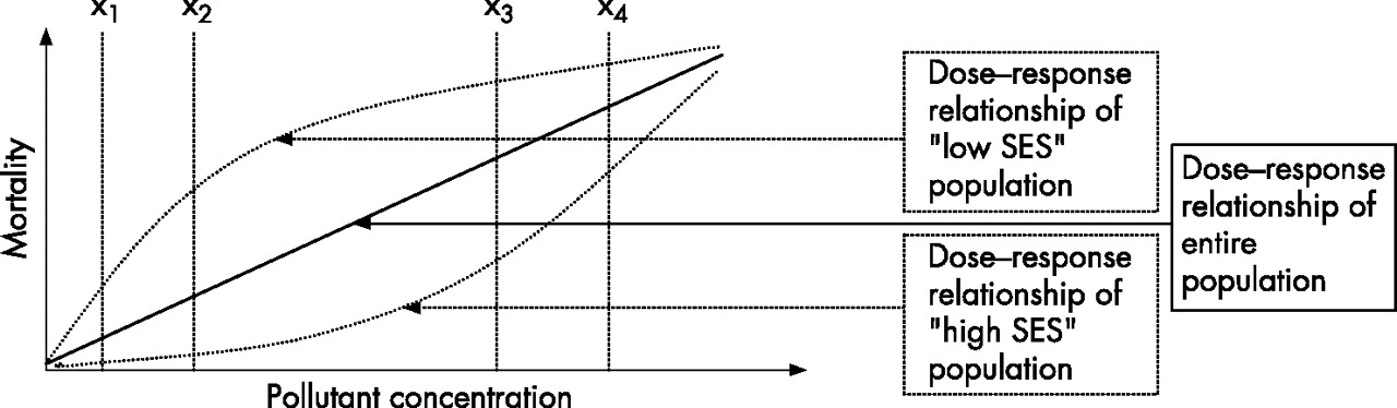
Each of the studies tested effect modification by SES only for a limited portion of the dose–response relationship between pollutant concentration and mortality. That is, in these studies, the relative risk is generally measured for an increase in the concentration of a pollutant (from concentration x₁ to concentration x₂). Some populations may conceivably be more susceptible than others to concentrations that are generally considered “low”. Other populations, less susceptible to these “low” concentrations, may become increasingly susceptible as the pollutant concentration increases. Figure 1 illustrates a fictitious example: the slope of a dose–response curve corresponding to a population with low SES might be stronger than that of a population with high SES for some concentration ranges (between x₁ and x₂), and lower for a range of higher concentrations (between x₃ and x₄). The slopes of these curves may be considered equivalent to relative risks. This shows the importance of taking into account the range of pollutant concentrations tested for which SES might be an effect modifier.

CONCLUSION

The available studies do not allow confirmation or exclusion of an influence of SES on the relationship between air pollution and mortality. More studies with comparable designs are necessary to achieve that aim.

Future studies must, in so far as possible, use exposure measurements that minimise differential exposure misclassifications according to SES. They must also test the largest possible number of SES indicators (individual and contextual, at different geographic resolutions)³¹ simultaneously to identify the most discriminating in terms of relative risks of mortality associated with pollution.

Additional multicentre studies would guarantee harmonisation of the indicators and statistical methods used.⁵⁹