We investigate the relation between government expenditures on public services and all cause mortality in US states (all figures for 1987), with emphasis on the part public services play in the relation between income inequality and population health. A large body of research now suggests that socioeconomic factors are influential in the production of population health,^1–4 and numerous studies have shown a relation between income inequality and mortality in the USA.^5–7

The causal factors underlying such a relation, however, have been debated.^5,10–17 One hypothesis is that places that tolerate high levels of income inequality may systematically underinvest in human capital and public services.¹³ Kaplan et al⁶ provided some preliminary evidence on this hypothesis, finding that lower state income inequality was associated with higher education spending (r = 0.32, p = 0.02) and library books per capita (r = 0.42, p = 0.002). This paper addresses the underinvestment hypothesis by examining: (1) the relation between expenditures on public services by state and local governments and all cause mortality, and (2) whether the association between income inequality and mortality is attenuated by public spending. Similar analyses have shown that in US central cities, the association between income inequality and premature mortality was robust to controls for public service expenditures.^8,9 These studies, however, did not control for between place differences in the cost of providing services, and may therefore misrepresent the level of services provided. Other research has suggested that the place-level relation between income inequality and population health is eliminated by the inclusion of controls for place-level racial composition or educational attainment.^18,19 But two recent multilevel studies showed that the relation between minority racial concentration and self rated health status was an artefact of the individual level relation between racial status and health. In other words, controlling for racial minority composition in ecological studies of this type inappropriately specifies an attribute of people as an attribute of places.^20,21

The focus on public goods in this paper follows from the notion of “real income” (or “effective income”), instead of cash incomes, with the former defined as: “all receipts which increase an individual’s command over the use of a society’s scarce resources”.²² The importance of effective income for health inequalities research is that it represents a person’s command over resources, whether or not those resources are purchased with cash incomes. Existing research on income and health focuses almost exclusively upon cash incomes, ignoring sources of effective income like public goods and services. It follows that the importance of cash incomes to health could, in principle, vary substantially from place to place, depending on the public goods and services to which citizens are entitled.

In this paper, the term public service refers to services provided by state or local governments. In most cases there are positive externalities associated with the provision of public services, even when the narrow definition of a “pure” public good is not met. A public good is defined by two criteria: (1) joint supply or non-rivalness, which means that once a good is supplied to one person, it can also be supplied to all other persons at no extra cost—a corollary to this is that one person’s consumption of the good does not affect consumption of the good by others; (2) non-excludability, whereby having provided a good to one person, it is impossible to exclude any person from consuming it, regardless of their willingness to pay (that is, through taxes or fees).²³ Classic examples of public goods include clean air and military defence. Many of the public services provided by governments are “impure” public goods, as they do not wholly satisfy these criteria, but their contribution to effective incomes may nevertheless be important.

Public services provided by state and local governments can be considered attributes of states. State level per capita public expenditures, however, measure what is spent on services, not the level of services consumed by residents. We also examine, therefore, expenditures that are adjusted for state by state variation in the cost of providing services to better represent the average level of services consumed in that state. This study cannot address the individual variation in consumption of public services (few studies can) because people have a tendency to underestimate their preference for public goods.^23,26,27 The practical implication of our focus on public goods is to widen the set of policy options to redress health inequalities. Such options may not be limited to redistribution of cash incomes, which some have argued are unjustified by available evidence,²⁸ but may also include the provision of public goods. Indeed, public goods may have efficiency advantages because of their joint supply attribute.²⁹

METHODS

Data for 1987 state level public expenditures were drawn from a report by the Advisory Commission on Intergovernmental Relations (ACIR),²⁴ and the US census of government.²⁹ The ACIR also estimated the cost of providing the US average level of public services in each state. Inequality in 1987 household income was measured using the Gini coefficient, calculated by the USA Census Bureau,³⁰ using data from the current population survey (CPS). The Gini coefficient varies between zero and one, with zero representing complete equality and one representing complete inequality. We have scaled the Gini to vary between 0 and 100. Median household income in 1987 was taken from the CPS,²⁵ and adjusted for between state differences in the cost of living.³¹ Finally, state level mortality rates, standardised to the 1970 US population, were acquired from the USA Department of Health and Human Services.³² Average direct general expenditures by state and local governments in the USA in 1987 were $2685 per capita,²⁴ or about 10% of the median household income of $25 986.²⁵

In the following analyses, we first examine associations between state level per capita expenditures on public services (total expenditures and by subcategory) and all cause mortality for three population groups (all ages, and both working age men and women). Secondly, we examine associations between mortality and two measures of public services. In the final stage of the analysis, we use multiple regression to determine if the relation between income inequality and mortality is conditioned on measures of public services. For all regression models, all two way interaction terms were calculated and tested for their contribution to the base models. None of the interaction terms made a significant contribution (F statistic was non-significant) to any of the models.

The index of public services we use to estimate the level of services consumed adjusts for the service “workload factors” in each state and inter-state variation in wages. The ACIR estimates “how much it would cost the governments in a state to provide the national-average (representative) level of services” by defining the state by state workload factors for each major expenditure area.²⁴ Because wages account for about half the cost of providing most public services, the estimates also take into account between state variation in wage rates, with the wage adjustment weighted differently for each expenditure subcategory, depending on the relative importance of wages²⁴ (see appendix). In other words, a state may have more than the average number of school age children per capita—a higher workload factor—but spend only the average per capita amount to provide education services. Other things being equal, children in that state will receive less than the average level of education services.

For example, average expenditures on primary and secondary education in the USA were $644.14 per capita in 1987. These expenditures serviced the 11.99% of the US population who were of primary school age, the 5.85% who were of secondary school age and the 5.67% who were children living in poverty (see table 1). However, Alabama had more than the average number of residents of primary and secondary school age, and more children living in poverty. Given these education workload factors, the “representative” expenditures necessary for Alabama to provide the US average level of education services was $695.24 per capita, higher than the US average, even after adjustment for below average wages in Alabama. In contrast, Minnesota had less than the average share of school aged children or children living in poverty, and wages slightly above the US average, resulting in representative expenditures slightly below the USA average.

A measure of the level of services in a given state relative to the USA average is provided by the ratio of actual expenditures (what was spent) to “representative” expenditures (what needed to be spent). The index of variation in this ratio (column (g) in table 1) shows that, other things being equal, the level of elementary and secondary education services provided to residents of Alabama was 60.5% of the US average while the level in Minnesota was 117.8% of the US average.

The ACIR’s estimates incorporate the best known reasons for variations in the cost of providing services. They are likely to better reflect the level of public services available to the average resident than do crude per capita expenditures.

RESULTS

Table 2 shows the correlations between key variables. Income inequality was significantly associated with higher mortality (r = −0.505, p<0.001) and lower median income (r = −0.501, p<0.001). In general, greater income inequality was associated with lower state expenditures on public services. Median state income was not strongly correlated with mortality, although higher median income was associated with higher public expenditure levels.

The upper left hand quadrant of table 3 shows Pearson correlation coefficients for the association between total and category specific per capita public expenditures (unadjusted) and each of three types of mortality rates. Figure 1 also shows the relation between higher per capita expenditures on public services and male working age mortality graphically (the circles representing each state are drawn proportionate to population size). Expenditures on primary and secondary education, higher education, highways, environment and housing, and general government administration were all significantly negatively associated with all age mortality and male working age mortality, while expenditures on both types of education as well as highways are significantly associated with female working age mortality as well. The bottom left hand quadrant of table 3 shows Pearson correlation coefficients for the index of public services and mortality rates. After adjustment for workload factors, education expenditures retained their significant association with all three mortality measures; associations between environment and housing and general government expenditures and male working age mortality reached statistical significance; associations between highway services and mortality were no longer significant and police and corrections services became significantly negatively associated with all cause, all age mortality and male working age mortality.

• Download figure
• Open in new tab
• Download powerpoint

Figure 1

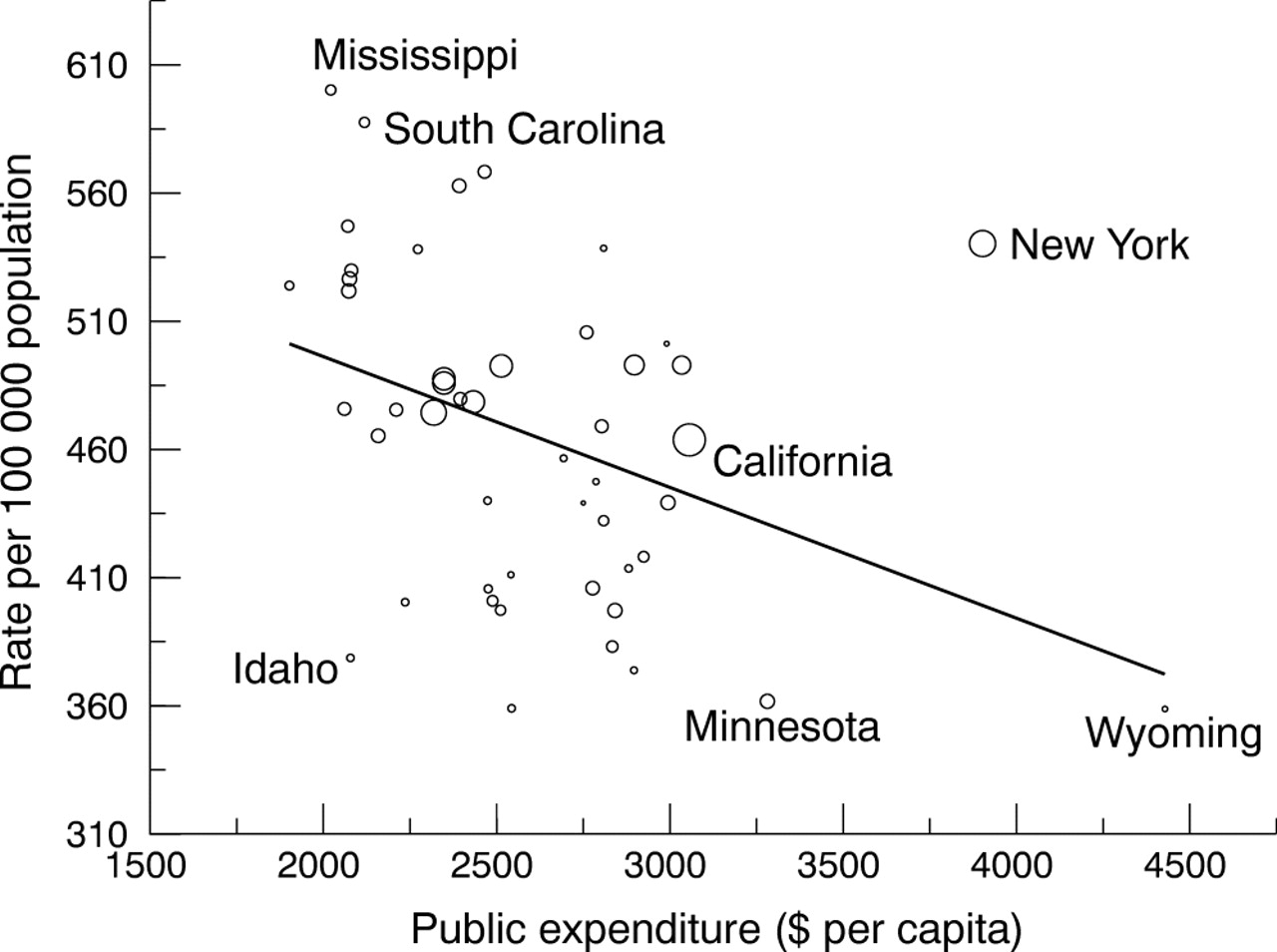
 Association between state level, per capita total expenditures on public services by state and local governments and working age (25–64) male mortality.

The right side of table 3 shows regression coefficients (with just one predictor variable) for the relation between per capita expenditures and the three mortality measures. These suggest that the relation between public services and mortality rates is strong, particularly for men of working age. Each additional $100 per capita in spending on higher education (the equivalent of $162.85 in 2003³³ and 3.8% of average state spending in 1987), for example, translates into a hypothetical reduction of 65.6 deaths per 100 000 in the male working age population. In 2001 terms, this is equivalent to the elimination of all deaths from accidental injuries, homicides, and diabetes combined.³⁴ Table 4 summarises the differences in the relation between each expenditure category before and after adjustment for wages and workload factors, by showing which cells showed no relation (NR) or a negative (−ve) relation between public expenditures/services and the mortality measure. Embolded cells show where adjustment for input costs and workload factors changed the relation. The table suggests that the relation between mortality and expenditures on public welfare, highways, police and corrections, and environment and housing are sensitive to adjustment for wages and workload factors. In other words, per capita expenditure on public welfare, for example, is unassociated with male or female working age mortality, but after adjustment, greater spending relative to the US average is associated with lower working age mortality for both sexes. This implies that if spending on public welfare comes closer to meeting an estimate of need, it is more likely to be associated with lower mortality.

A number of other expenditure categories were significantly associated with mortality, but for some, adjustment for workload factors changed the result. Unadjusted expenditures on highways were negatively associated with mortality, but after adjustments (for vehicle miles travelled, miles of lanes/streets and roads not on federal land and labour costs), the relation disappeared. Public expenditures on police and corrections were negatively associated with total and male working age mortality, but only after adjustment for workload factors. Environment and housing expenditures were negatively associated with mortality in most instances, especially after adjustment for workload factors. This expenditure category includes natural resources, parks and recreation, housing and community development, sewerage and sanitation. Expenditures by state and local governments on health and hospitals were unrelated to mortality rates, even after adjustment for workload factors.

The final stage of the analysis examines whether the relation between income inequality and mortality is attenuated by public expenditures/services. The first two rows in each section of table 5 show regression coefficients for median income and the Gini coefficient each modelled alone. The third row shows that the relation between income inequality and mortality is robust to control for median income, consistent with previous studies.^6,35 Moreover, the strength of relation between the Gini and mortality is large: a one point increase in the Gini translates into an additional 22.8 deaths per 100 000 for male working age mortality (in a model with an R² over 0.40). The introduction of selected measures of public expenditures and services attenuates the effect of income inequality a modest amount. After controlling for median income and the Gini, a $100 increase in unadjusted total public expenditures per capita translates into roughly 3.9 fewer deaths per 100 000 population (all age, all cause mortality). Similarly, a one point rise in the index of public services is associated with a reduction of 0.8 deaths per 100 000. Finally, per capita expenditures on education (primary, secondary and higher education combined) are strongly associated with mortality. Each additional $100 per capita expenditure on education (combined elementary, secondary and higher education) translates into 23.5 fewer deaths per 100 000 among working age men, even after controlling for median income and income inequality. In all cases, the relation between public expenditures and mortality are strongest for working age men.

DISCUSSION

We found that the relation between income inequality and mortality was modestly attenuated by the addition of measures of public services to our models. In other words a portion of the relation between income inequality and mortality may be attributable to consumption rights embodied in public services provided by state and local governments. This implies that if, as some have argued,^13,17 income inequality is a marker for other factors with a more direct causal relation to mortality, the (under)provision of public goods and services is only a part of the putative bundle of factors that income inequality summarises.¹⁷ One possible caveat to this interpretation, however, is that rather than being a causal factor in the model, public expenditures may act as a partial confounder in the relation between income inequality and mortality. In addition, it is also possible that the workload adjustments fail to accurately depict the relative need for services. For example, the relative weights assigned to each workload factor by the ACIR²⁴ may be inaccurate. The fact that expenditures on public services are significantly related to mortality underlines the need to develop the best possible measure of the average services consumed by residents of a jurisdiction.

With respect to our first objective, we found that the provision of public services by state and local governments was strongly related to state level all cause mortality rates, with especially strong associations with male working age (25–64) mortality. Public expenditures on education (both elementary/secondary and higher education) seem to have the most profound impact on state mortality rates. This is consistent with the well established in previous research that for individuals, greater educational is a strong protective factor for health.^36,37 The stronger association between higher education and mortality may be because higher education has its greatest effects on those young adults who are at greatest risk for premature mortality from accidents, suicides, and homicides, so to the extent that greater opportunities for a college education results from higher expenditures, this may reduce exposure to such risks. One important note, however, is that there may be state by state variation in the proportion of students educated in the public school system. If the tendency for students from affluent families opt out of the public school system (in favour of religious and/or private schools) differs systematically from state to state, this may create pressure to reduce taxes, reduce spending, but leave behind disproportionately high number of disadvantaged students and distort the relation between public spending on education.

As expected, greater expenditures on public welfare were associated with lower mortality rates, although only after adjustment for workload factors. Expenditures on police and corrections were also associated with lower male working age mortality, after adjustment for workload factors. Finally, expenditures on environment and housing were associated with lower female working age mortality, after adjustment. It is possible that young women benefit from expenditures on public housing because it provides an environment with fewer mortality risks than private rental housing (although public housing is clearly not without risks). The absence of any effect of expenditures on health and hospitals has at least two possible explanations, but the measure is not specific enough to distinguish them. On the one hand, it is consistent with international comparisons of health spending and life expectancy, which are weakly related,³⁸ and not inconsistent with estimates that about half of the gain in US life expectancy in the second half of the 20th century can be attributed to advances in modern medicine.³⁹ On the other hand, there is evidence that greater access to primary care (especially family physicians, but not most specialty care) is associated with better population health in the USA and elsewhere.^40–44 This raises the possibility that spending on health and hospitals by state and local governments is a poor indicator of access to medical care and does not capture the positive population health effects of access to primary care, especially access to family medicine practitioners.

There are some important limitations to our analysis. Firstly, in all cases, spending on public services, even with adjustment for workload factors, is only a good measure if expenditures on services that influence health and are distributed equitably. Moreover, we have treated individual expenditure categories as independent from one another. With a larger number of observations (for example, counties), you could investigate the optimal mix of service expenditures. This is important because most expenditure decisions are made within a near fixed budget, and it would be beneficial to know the health “costs” of certain spending trade offs. A second limitation of our analysis is that we have used essentially just one indicator of population health, mortality. Previous studies have shown that the relation between income inequality and health may be sensitive to the choice of health measure.^7,41

Our findings suggest that public investments in services related to education, environment and housing, police and corrections, and public welfare may be beneficial to population health, so long as they are adequate to meet the needs of the local population and overcome unique aspects of the service delivery environment that may raise the costs of providing services (like wages). Moreover, the relation between public goods expenditures and mortality seems to be partly independent of the effects of income inequality. These findings underscore the argument that an exclusive focus on the relation between cash incomes and health is insufficient, and that a more complete approach embraces the notion of effective income as a health determinant, one component of which is command over resources people have as a result of the provision of public goods. It follows that the policy options to address the possible effect of income inequality on health are not limited to redistributing cash incomes using such instruments as transfer payments and tax credits, but also include public spending on policies and services that have the potential to increase people’s command over resources, or effective income. From our analysis, the most promising sectors for public investment to improve health are higher education and primary and secondary education. So long as such expenditures are able to produce high levels of equitably distributed services (overcoming input cost and “workload factors”), our findings suggest one would expect an impact on population health.

APPENDIX

The relative services index (or adjusted expenditures measure) was developed by the Advisory Commission on Intergovernmental Relations²⁴ to allow for between state differences in the cost of providing a level of services equal to the US average. Different adjustments, however, are applied to the various categories of expenditure. All expenditure categories were adjusted for population size and by the average wages of male workers aged 45 to 54 (controlling for educational attainment) and weighted by the estimated proportion of total costs that wages represent in the public service subcategory. In addition to adjustment for population and wages, for several categories, the commission derived “workload” factors—additional factors that contribute to between state differences in the cost of providing the US average of public service—by reviewing the literature and consulting with public finance experts in each area. For primary and secondary education the workload factors were: proportion of the population of elementary school aged (weight 0.6), and secondary school aged (weight 1.0) (children in private school deducted from these numbers), and the proportion of children under 18 living in households below the poverty line (weight 0.25). For higher education, workload factors were the weighted sum of population of different age groups, weighted by their educational participation rate. For public welfare, the lone workload factor was the proportion of the population living in households below the poverty line. For health and hospitals the factors were the equally weighted sum of population age 16–64, population with disabilities and proportion of the population living in households below 150% of the poverty line. For highway expenditures the factors were the weighted sum of vehicle miles travelled and lane/streets and roads not on federal land. For police and corrections the factors were the equally weighted sum of proportion of the population aged 18–24 and the murder rate. For further details, see Rafuse.²⁴