Article Text

Abstract
Study objective: This didactical essay is directed to readers disposed to approach multilevel regression analysis (MLRA) in a more conceptual than mathematical way. However, it specifically develops an epidemiological vision on multilevel analysis with particular emphasis on measures of health variation (for example, intraclass correlation). Such measures have been underused in the literature as compared with more traditional measures of association (for example, regression coefficients) in the investigation of contextual determinants of health. A link is provided, which will be comprehensible to epidemiologists, between MLRA and social epidemiological concepts, particularly between the statistical idea of clustering and the concept of contextual phenomenon.
Design and participants: The study uses an example based on hypothetical data on systolic blood pressure (SBP) from 25 000 people living in 39 neighbourhoods. As the focus is on the empty MLRA model, the study does not use any independent variable but focuses mainly on SBP variance between people and between neighbourhoods.
Results: The intraclass correlation (ICC = 0.08) informed of an appreciable clustering of individual SBP within the neighbourhoods, showing that 8% of the total individual differences in SBP occurred at the neighbourhood level and might be attributable to contextual neighbourhood factors or to the different composition of neighbourhoods.
Conclusions: The statistical idea of clustering emerges as appropriate for quantifying “contextual phenomena” that is of central relevance in social epidemiology. Both concepts convey that people from the same neighbourhood are more similar to each other than to people from different neighbourhoods with respect to the health outcome variable.
- ICC, intraclass correlation
- SBP, systolic blood pressure
- MLRA, multilevel regression analysis
- VPC, variance partition coefficient
- blood pressure
- multilevel analysis
- neighbourhood health
Statistics from Altmetric.com
- ICC, intraclass correlation
- SBP, systolic blood pressure
- MLRA, multilevel regression analysis
- VPC, variance partition coefficient
This article has, on the one hand, didactic purposes and is directed to readers disposed to approach multilevel regression analysis (MLRA) in a more conceptual than mathematical way. Readers who wish an alternative or more formal statistical explanation may consult any of the other references on multilevel analysis published elsewhere.1–5
On the other hand, and perhaps more important, in this essay we also develop a vision of multilevel analysis6 that considers measures of health variation7 (for example, neighbourhood variance, intraclass correlation) for understanding the distribution of health in the general population rather than only applying measures of association (for example, regression coefficients, odds ratios)8 to understand contextual determinants of individual health. We believe that, so far, measures of health variation have been underused in multilevel epidemiology.
Our aim is to provide a link, which will be comprehensible to epidemiologists, between MLRA techniques and social epidemiological concepts, particularly the analogy between the statistical concept of clustering and the social epidemiological idea of contextual phenomenon.
It is intuitive that people from the same area may be more similar to each other in relation to their health status than to people from other areas. In other words, persons with similar characteristics may have different degrees of health according to whether they live in one area or another because of differing cultural, economic, political, climatic, historical, or geographical contexts.9 This contextual phenomenon expresses itself as clustering of individual health status within areas. That is, a portion of the health differences among people may be attributable to the areas in which they reside.6,10
The notion of contextual phenomenon has a long history in epidemiology and is included under different forms in the Durkheimian concept of social fact,11 Rose’s notion of population disease rates,12,13 and John Snow’s findings on cholera incidence.14 These three related seminal conceptions are contextual in their nature, and support the idea that knowledge on the distribution and determinants of population health is epistemologically multilevel15 and needs to consider both people and areas.10,16,17
The idea of contextual phenomenon, which could be considered as a core notion in social epidemiology, corresponds to the statistical concept of clustering*—that is, in turn, the main reason for applying multilevel regression techniques. Statistically, it is necessary to use techniques that, like MLRA, consider the dependence of the outcome variable between people from the same area. An important assumption made in usual regression analyses is the independence of individual measures. If this assumption is violated, the results of the regression analysis are biased.1 However, we have previously emphasised6 that clustering of individual health within neighbourhoods is not a statistical nuisance that only needs to be considered for obtaining correct statistical estimations, but a key concept in social epidemiology that yields important information by itself.2,6,19–21 The more the health of the people within a neighbourhood is alike (as compared with people in other neighbourhoods), the more probable it is that the determinants of individual health are directly related to the contextual environment of the neighbourhood, and/or that social processes of geographical segregation are taking place—that is, similar types of people choose or are forced to reside in a given neighbourhood.
Those aspects are of high significance in social epidemiology as they have value in the context of ideas about the efficacy of focusing intervention to reduce health inequalities on certain geographical areas rather than on specific people only. Measures of variation are important in public health to understand the significance of specific contexts for different individual health outcomes.7 Traditional measures of association, in contrast with measures of variation, do not inform on the multilevel distribution of health.6
Without being a panacea to miraculously fix the ills of a “risk factor” epidemiology that seems inappropriate for assessing the impact of the context,23 MLRA is a suitable statistical technique that can be used to operationalise conceptual schemas in multilevel epidemiology.
In this essay we explain how to investigate whether a given health phenomenon (for example, systolic blood pressure) has a contextual dimension. Using this research question, we introduce the “empty” MLRA model. This model is the simplest form of MLRA as it does not include any covariate but focuses only on how health differences are distributed between people and between areas. Along the explanation of the empty model, we present figures that permit a visual comprehension of MLRA concepts such as residuals, partitioning of variance at different levels, and the idea of clustering and intraclass correlation.
THE “EMPTY” MLRA MODEL
To explain MLRA we use an example based on hypothetical data. The population of the example consists of 25 000 subjects, 35 to 64 years old, living in the 39 neighbourhoods of an imaginary city. The individual outcome variable is systolic blood pressure (SBP), and we assume that it is continuous and follows a normal distribution. As this article explains the empty MLRA model, we do not use any independent variable but focus only on the mean and variance of SBP.
The example was adapted from a real empirical investigation that analysed countries rather than neighbourhoods.10 This essay is based on simulated data and, therefore, the results presented in this article should not be used as empirical evidence. For all analysis, we use the software MLwiN version 1.1 developed by Goldstein’s research group†.24
The reason for naming this model “empty” is that it does not include any explanatory variables but only estimates the city SBP mean and the neighbourhood and individual differences in SBP on the basis of the study sample. We present below a very simple equation of the model that will be clear to readers not trained to read formal statistical notations. Readers who wish a formal statistical explanation are referred elsewhere.2,25,26
SBPI = SBPC+EN−c+EI−c
SBPI = SBP of an individual in a neighbourhood
SBPC = Mean SBP of the city
EN−c = Difference between the city SBP mean and the neighbourhood SBP mean (also known as neighbourhood “shrunken residual”)
EI−c = Difference between the neighbourhood SBP mean and the individual SBP value (also known as “individual residual”)
In MLRA both people and neighbourhoods are assumed to be randomly sampled from a population of persons and a population of neighbourhoods. It is assumed that the residuals are normally distributed and that there is independence between the individual residuals and the neighbourhood residuals. MLRA presents advantages compared with the common analysis of variance.
The model presented above shows that the SBP value of a person living in a neighbourhood (SBPI) is equal to the mean SBP in the city (SBPC) plus the predicted neighbourhood difference from the city mean (that is, neighbourhood shrunken residual [EN−c]) plus the individual difference from the neighbourhood mean (that is, individual residual [EI−c]).
Partitioning overall differences in SBP
The presence of neighbourhood and individual residuals in the empty multilevel model just shows that SBP varies both at the individual and at the neighbourhood level. The main intent of the empty model is to partition the total variance in SBP in the city (VTotal) into a variance that occurs between neighbourhoods (VN) and a variance that occurs between people (VI) as shown in the equation 1, illustrated in figure 1, and calculated in table 1.
Multilevel, individual and ecological linear regression analysis of systolic blood pressure (SBP) in 25 000 people living in the 39 neighbourhoods (hypothetical data)
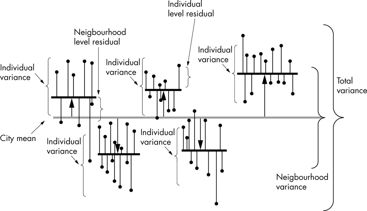
Multilevel information. In this figure the neighbourhood residuals are represented by the length of the pillows between the city SBP mean, represented by a grey colour, and the neighbourhood SBP means represented by thick black horizontal lines. The individual residuals are represented by the length of the vertical lines between the neighbourhood means and the individual SBP values represented by black circles at the top of thin lines. In this figure we do not have any explanatory variable (that is, this figure corresponds to an “empty” model) as we are only interested in analysing how individual blood pressure differences are partitioned in a variability that exists between people from the same neighbourhood and a variability that exists between neighbourhoods. In this figure we can imagine that the neighbourhood means (short thick lines) pull up or pull down all the individual SBP values belonging to the same neighbourhood, even if individual level variability remains within neighbourhoods. The mathematical expression of the intraclass correlation can be visually understood in figure 1. Figure 1 is a graphic combination of figures 3 and 4.

In figure 1 we can visualise the empty model and the concepts that it conveys. In this figure the neighbourhood differences from the city mean represent the shrunken residuals. The figure shows that multilevel structures convey information on variability both between and within neighbourhoods. The variance is a summary of the differences. The higher the variance, the larger the differences are. In figure 1 the brackets show that the total variance is the sum of the between neighbourhood variance and the within neighbourhood variance.
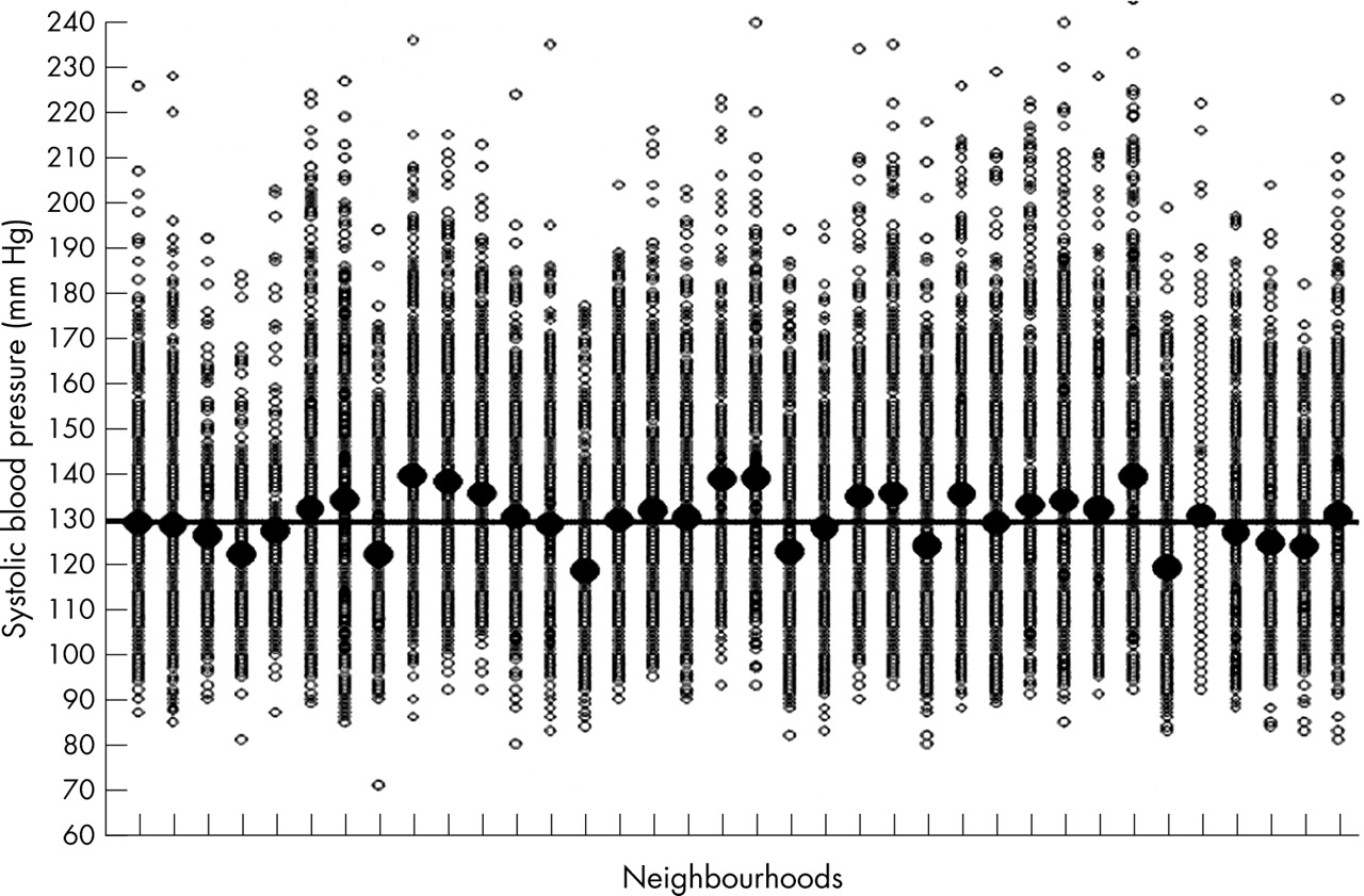
Figure 2 shows the individual and neighbourhood SBP values used in our example. We can see that each neighbourhood has a specific SBP mean (black dots) that differs from the city mean (130 mm Hg) by a certain amount of mm Hg. This difference is the neighbourhood level raw residual.

The figure shows the actual SBP values used in our example. The large black dots represent the neighbourhood means. The small circles represent the individual SBP values within neighbourhoods. The horizontal black line represents the city SBP mean.
Single level individual studies compared with MLRA
In table 1 we can see that the empty model gives evidence of both between individual (VI = 433.4) and between neighbourhood (VN = 36.2) variance in SBP. If we combine the variance from both levels to give a total variance, we see that this total variance (VTotal = 468.1) is similar to the variance obtained by a simple individual level analysis using descriptive statistics. Reading table 1, you can understand intuitively that a portion of the individual level variance is in fact neighbourhood level variance.
Imagine that figure 3 represents the distribution of individual SBP in the population of the city described in the example. As in individual single level analysis we have individual data only, the fact that people are grouped within neighbourhoods is neglected. In figure 3 we merely see differences between the individual SBP values and the mean SBP value of the whole city (the single level individual residuals). We are unable to distinguish the differences between the mean blood pressure in each neighbourhood and the overall mean blood pressure in the city. In single level individual based designs, we tend to neglect possible neighbourhood effects. This oversimplified approach has been termed the individualist fallacy.27
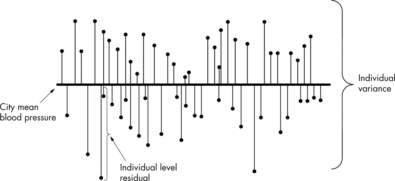
Single level individual information. This figure represents the distribution of individual SBP in the population of the city when we have only single level individual based information. The fact that people are grouped within neighbourhoods is neglected, as we only have individual level data. In this figure the length of the thin vertical line from the black spot to the thick horizontal line represents the individual differences in blood pressure compared with whole city mean (the individual level residuals). The individual variance in single level individual studies is an average summary of these differences. In single level individual analysis we consider all information as if it were at the individual level neglecting possible neighbourhood components.
Single level ecological studies compared with MLRA
Table 1 also shows the between neighbourhood variance obtained by an ecological analysis performed by aggregation of the individual SBP values at the neighbourhood level. In the ecological analysis we estimate the mean SBP for each neighbourhood from the sample of people in each neighbourhood, and then we compute the variance of these estimated means. The ecological variance computed in this way overstates the neighbourhood variance because it also includes variation attributable to sampling error (imprecision) in the estimates of each neighbourhood mean SBP.
The ecological variance is rather similar to the between neighbourhood variance in SBP obtained by the MLRA. It is patently clear that the single level ecological analysis neglects the existence of individual level variance. Figure 4 illustrates that in an ecological analysis we are unable to observe differences between people (variation in blood pressure within a neighbourhood), but we can distinguish differences between the mean blood pressure of each neighbourhood and the mean blood pressure of the whole city (that is, the neighbourhood residuals of an ecological analysis).
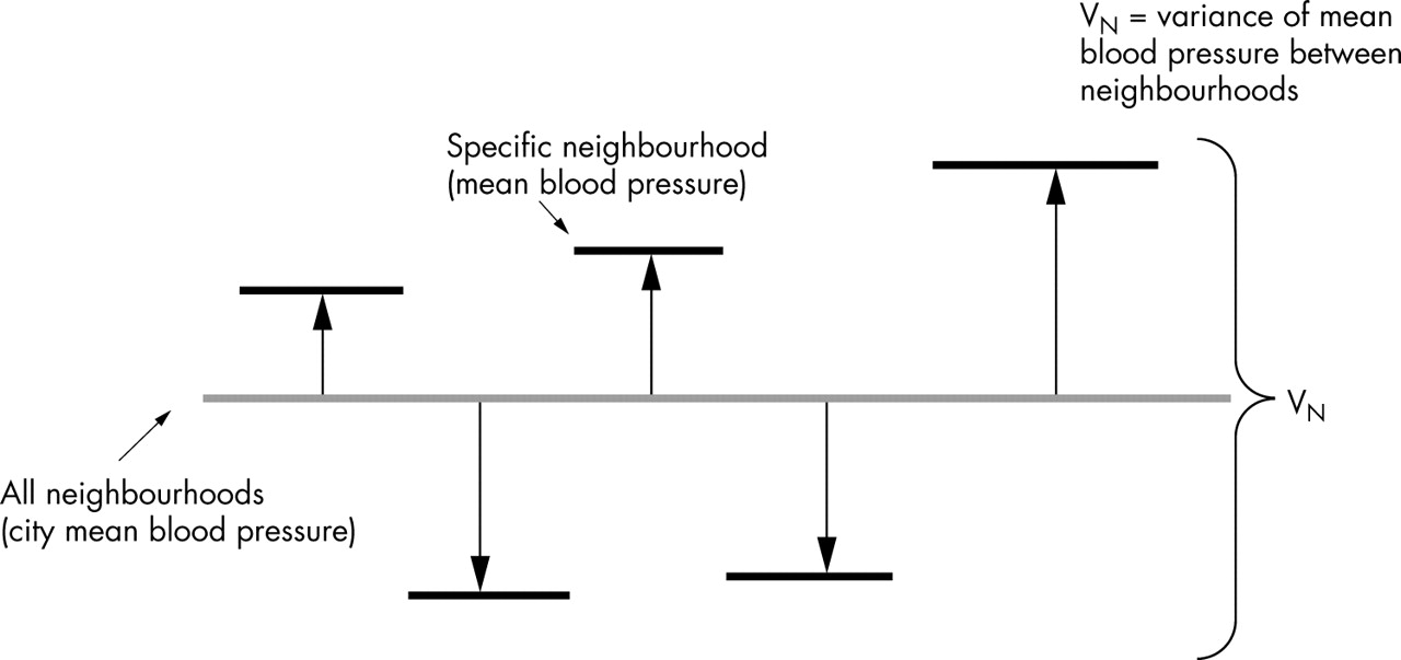
Single level ecological information. In this figure all individual SBP values are aggregated at the neighbourhood level to obtain the neighbourhood mean. We can distinguish differences between the mean blood pressure of each neighbourhood and the mean blood pressure of the whole city (the neighbourhood residuals). These residuals are represented by thick black horizontal lines at the top of a pillow. The neighbourhood variance is a summary of the differences between neighbourhoods. We are unable to observe differences between people (variation in blood pressure within neighbourhoods). In single level ecological analysis we consider all information as if it were at the neighbourhood level neglecting individual components.
In single level ecological analysis, we consider all information as if it were at the neighbourhood level, neglecting possible individual components (this oversimplified approach has been termed the sociological fallacy).27
Today it is well known that neither single level individual nor ecological analyses are suitable for effectively investigating contextual effects.22
The intraclass correlation (ICC) or variance partition coefficient (VPC)
It is seen in figure 1 that all people living in the same neighbourhood share a common level of blood pressure that differs from the city mean in an amount that corresponds to the neighbourhood residual. Therefore, we often speak about “differences between neighbourhoods” and “differences between people within neighbourhoods”. Together the individual and the neighbourhood variance components represent the total differences in SBP. We can see that a portion of the total individual SBP difference is at the neighbourhood level, and in the empty model we can quantify this aspect by computing ICC. As equation 2 shows, the multilevel ICC is the proportion of the variance in SBP that occurs at the neighbourhood level. In this sense the ICC is a variance partition coefficient (VPC).1
It can be seen in figures 3 and 4 that in single level analysis we are unable to calculate the ICC, because information on how variance is partitioned at different levels is not available.
The ICC equation is intuitive and can also be understood by observing figure 1.

In this formula VI is the variance between people from the same neighbourhood (1st level variance) and VN is the variance between neighbourhoods (2nd level variance).
As variance can only be positive, according to equation 2 the ICC is necessarily between 0 and 1. Table 1 shows that the ICC, which measures individual SBP clustering at the neighbourhood level, is equal to 0.08. Therefore, in our example 8% of the total individual differences in SBP are at the neighbourhood level. On these grounds, we might conclude that there is some evidence for a possible neighbourhood contextual phenomenon shaping a common individual SBP level. Alternatively, this clustering might be attributable to the different composition of neighbourhoods.
The name “correlation” suggests that the ICC expresses the similarity in health status (in our example SBP) between two persons in the same neighbourhood. An ICC equal to 1 would inform us that all the people in a neighbourhood have an identical SBP level (that is, 100% of the total individual differences are at the neighbourhood level), and an ICC equal to 0 that the people do not share any neighbourhood related common level of SBP.
A high ICC value informs us that neighbourhoods are very important in understanding individual differences in health. On the other hand, an ICC of 0 would suggest that the neighbourhoods are similar to random samples taken from the city and suggest that neighbourhoods are not relevant to understanding SBP differences. Snijders also gives a didactic example of this concept (page 18).2 When the ICC is 0, the suitability of performing a multilevel analysis is less obvious. In the absence of a multilevel structure, a single level individual analysis is appropriate.
We may be interested in knowing if the ICC is statistically different from 0. The simplest method would be to perform a statistical test of the neighbourhood variance.1–3 When the neighbourhood level variance is not significant, there is no justification for computing the ICC. However, when testing the neighbourhood variance you need to consider the statistical power in MLRA considering that it depends more on the number of neighbourhoods than on the number of people.2 Remember that absence of evidence is not evidence of absence.28
If the ICC is 0, it does not necessarily mean that the neighbourhood context is not important compared with individuals’ factors. Rather, an alternative reason could be that the geographical boundaries we use to define the actual neighbourhoods do not correspond with the boundaries that shape the relevant environment for the concrete individual health outcome. An ICC close to 0 in an empty model may hide considerable neighbourhood variability that would only appear in more complex models. Moreover, a small ICC does not prevent the existence of significant associations between neighbourhood variables and individual health as comparatively small variance between neighbourhood means may give enough contrast of exposure to detect associations.6,25 These aspects are more extensively discussed in companion papers.29,30
What this paper adds
-
We provide a link—comprehensible to epidemiologists—between multilevel regression techniques and social epidemiological concepts, particularly the analogy between the statistical concept of clustering and the social epidemiological idea of contextual phenomenon.
-
We develop a vision of multilevel analysis that considers measures of health variation (for example, neighbourhood variance, intraclass correlation) for understanding the distribution of health in the general population rather than only applying measures of association (for example, regression coefficients, odds ratios) to understand contextual determinants of individual health.
-
Measures of health variation have been underused in multilevel epidemiology.
-
Statistical measures of clustering emerge as appropriate for quantifying “contextual phenomena”, which is of central relevance in social epidemiology.
“Shrunken” neighbourhood level residuals
An extra comment on how neighbourhood level residuals are calculated in MLRA is necessary as these residuals are often used in epidemiology and community health studies to rank second level units (for example, hospitals) and investigate geographical differences in health.31–33
In the simplest case, the raw residual is the difference between the city and the neighbourhood mean SBP. The shrunken neighbourhood residual (EN−c) obtained with the multilevel regression is then calculated a posteriori by multiplying the raw neighbourhood residual by a shrinkage factor (SF) shown in equation 3:

Obviously SF has a value between 0 and 1. The neighbourhood “shrunken” residual is calculated by weighting the raw residual with SF as in equation 4:

The neighbourhood “shrunken residuals” are computed using the raw residuals, the estimated variances, and the number of people in the neighbourhood (Nn). MLRA can be performed even when the number of people (1st level units) within each neighbourhood (2nd level unit) is very different. The fewer the number of people in a neighbourhood, or the higher the variability within neighbourhoods as compared with the variability between neighbourhoods, the more important the shrinkage and the more the value of the neighbourhood residual will be shrunken towards 0. The value (SBPc+EN−c) is also termed “posterior mean”.1
Computing these shrunken residuals may be viewed as disentangling the proportion of each residual that may be attributed to true variations between neighbourhoods from that proportion that might better be attributed to random variations.34 Rather than only considering the neighbourhood level variance as a summary of the variations that exist between neighbourhoods, the shrunken residuals inform how each specific neighbourhood differs from the city mean.
Policy implications
-
It is important that political decisions are grounded in appropriate analysis. This study explains a modern methodology of analysis that can be applied in this context.
-
Multilevel analyses can be used to identify the relevance of the neighbourhood or other societal boundaries for understanding health inequalities.
-
Our study has value in the context of ideas about the efficacy of focusing intervention to reduce health inequalities on certain geographical boundaries rather than on people only.
-
Politicians should always consider the fact that the health of the citizens may depend on their context, which deserves to be investigated and accounted for when planning public health interventions.
In figure 5 we have ranked the neighbourhoods according to their shrunken residual as explained above. The raw residuals are represented by white circles and in our example are very similar to the shrunken residuals due to the high number of individuals in each neighbourhood. The bars around each neighbourhood residual represent the 95% confidence intervals. It can be concluded that in these hypothetical data many of the neighbourhoods present a SBP that differs from the city SBP mean (represented by a dotted line).

Here neighbourhoods are ranked according to the mean SBP using the whole city mean SBP as reference in the comparisons. The neighbourhood values are the “shrunken residuals” (black circles) and the raw residuals (white circles). We provide 95% confidence intervals obtained in the multilevel regression analysis.
CONCLUSIONS
We have shown in a basic way that the simple investigation of how differences in SBP are partitioned between the individual level and the neighbourhood level provides relevant epidemiological information. Both the statistical idea of clustering (that is, ICC) and the social epidemiological concept of contextual phenomenon convey that people from the same neighbourhood are more similar to each other than to people from different neighbourhoods with respect to the health outcome variable. For this reason epidemiological measures of clustering as the ICC emerge as appropriate for identifying and quantifying “contextual phenomena”,6,35 which is of central relevance in social epidemiology.6,7,36
In companion articles we explain more complex MLRA models that include individual and neighbourhood level variables.29,37 In these articles we illustrate that the importance of the context for understanding health differences may differ for people with different characteristics. We also clarify that contextual factors may modify the effect of individual characteristics on health, and that individual and contextual factors can be used to explain compositional and contextual neighbourhood differences in health. We explain that measures of association between contextual characteristics and individual health, being important for understanding multilevel causal pathways, do not allow for assessing the multilevel distribution of health outcomes.
Studying multilevel health variation presents comparatively few complications and yields measures that are intuitively easy to understand when the outcome of interest meets the conditions for linear regression analysis. However, when the outcome is not continuous, interpreting measures of variation is less easy and it is the subject of this investigation.38,39 Appropriate measures are, however, already available,20,35,40–43 and we explain these measures in a companion paper. In any case, most epidemiological concepts that can be operationalised by multilevel linear regression analysis are of general validity and can be applied to any type of health outcomes.
Our essay may help to provide more insight into the use of measures of health variation based on the random effects of the multilevel models, and emphasise the decisive part they should play in social epidemiology and community health research. Statistical measures of clustering emerge as appropriate for quantifying “contextual phenomena”, which is of central relevance in social epidemiology.
Acknowledgments
We thank Klaus Larsen for his comments on the manuscript and Beatriz Gonzalez Lopez-Valcarcel and other anonymous referees for their constructive critics.
REFERENCES
Footnotes
-
↵* According to the ideas of Durkheim (1858–1917) people belonging to a specific community share a collective conscience (common social values and norms that are formed by human relations and interactions and that generate collective feelings of solidarity and connectedness). This collective conscience operates creating what Durkheim called “social cohesion” to bind the social structure together. Understood in this way, the social group emerges as an independent social fact rising over and above individual circumstances, and going beyond the sum of the people that compose it.11 Thus collective characteristics shape the health of the population in a way that cannot be reduced to individual characteristics. A classic example concerns population differences in suicide rates. Even if within each area the people at risk of committing suicide are not the same in different time periods, the differences between populations in suicide rates are fairly stable over time. This fact suggests the existence of a contextual phenomenon that conditions a clustering of individual suicide risk within areas. In other words, some part of the total differences in health between people might be as a consequence of the differences between the areas where the people live. Analogous consideration can be made when interpreting John Snow’s findings on cholera incidence in different areas of London14 and the ideas of Geoffrey Rose on sick people and sick populations.10,12,18
-
↵† For a review on other programs suitable for MLRA see the Centre for Multilevel Modelling, Institute of Education, London (http://multilevel.ioe.ac.uk/softrev/index.html).
-
Funding: this study is supported by grants from FAS (Swedish Council for Working Life and Social Research) for the projects “Development and application of multilevel analysis in pharmacoepidemiology and social medicine” (principal investigator: Juan Merlo, number 2002-054) and “Socioeconomic disparities in cardiovascular diseases - a longitudinal multilevel analysis” (principal investigator: Juan Merlo, number 2003-0580).
-
Competing interests: none declared.
Linked Articles
- In this issue