An aspect of central importance in social epidemiology is that the health differences between people can partly be attributed to the areas in which they live.^1–3 People with similar characteristics who live in different neighbourhoods may have different health statuses because of differing cultural, economic, political, historical, or geographical influences. In other words, different people may to some extent share similar health statuses because they share a common environment.⁴ This contextual phenomenon expresses itself as the clustering of individual health status within neighbourhoods.^5–7 The presence of clustering is, in turn, the main reason for applying multilevel regression techniques. If the individual health status is correlated within neighbourhoods, analysis using common regression methods underestimates the standard errors for contextual effects and gives biased results. Multilevel regression analysis (MLRA) is a statistical methodology that provides information on how health disparities are distributed between the individual and the neighbourhood levels, quantifies the clustering of individual health status within neighbourhoods, and permits examining cross level interactions between the effects of neighbourhood and individual level factors.^8,9,10,11

Using an hypothetical example on systolic blood pressure (SBP), we have previously explained that MLRA can be used to investigate neighbourhood disparities in health without considering any specific neighbourhood characteristic but only the neighbourhood affiliation of each person.^12,13 A feature of those previous analyses was that the characteristics of the neighbourhood context remained unspecified. In MLRA, neighbourhood effects can actually be assessed by quantifying and modelling health differences, or variance, alone.

In this essay we go one step further in using MLRA to build an understanding of how this contextual phenomenon operates. We explain that neighbourhood differences in SBP can be accounted for by specific contextual characteristics such as the income level of a neighbourhood. This socioeconomic contextual characteristic may affect individual health over and above individual socioeconomic characteristics. We show that classic measures of association (for example, regression coefficients) between specific neighbourhood characteristics and health might help to elucidate possible cross level causal pathways. We also show how to investigate whether neighbourhood factors modify the effect of specific individual variables. We finally explain why those measures of association need to be interpreted together with measures of variance to improve our understanding of geographical health disparities.

POPULATION AND METHODS

The hypothetical example

Our hypothetical population consists of 25 000 subjects 35 to 64 years old, living in the 39 neighbourhoods of an imaginary city. There is a clear multilevel structure with individuals (level 1) nested within neighbourhoods (level 2). The individual outcome variable is SBP. For the didactic purpose only four individual variables were included: (1) age in years, (2) body mass index (BMI) in kg/m² (these two variables have been centred on their overall means of 49 years and 25 kg/m², respectively), (3) whether any antihypertensive drug (AHD) was used, and (4) individual low income defined as having an income under the median in the city. The neighbourhood low income was defined as having an average income under the median neighbourhood income in the city.

Our hypothetical study model was adapted from an empirical investigation, published elsewhere, analysing countries rather than neighbourhoods.¹⁴

MLRA

In this paper we follow a sequence of analysis that we also used in two previously published articles.^12,13 In these articles we described an “empty”* MLRA model (model i),¹² a model including individual variables only (model ii), a model with a random slope† for BMI (model iii), and a model further taking into account a non-constant individual variance‡ related to BMI (model iv).¹³

This paper completes the sequence of analysis described in previous publications^12,13 by including information on individual and neighbourhood socioeconomic position (that is, income), which permits disentangling their specific effects on SBP level.

In model iv⁰, which is a simple extension of model iv described in detail in a previous companion article,¹³ we additionally include individual low income. In model v we further introduce neighbourhood low income. In model v⁰ we expand model v by including a term for interaction between individual BMI and neighbourhood low income effects. This last model allows us to examine whether the effect of BMI on SBP is more intense in low income neighbourhoods or, to say things in another way, whether SBP differences between low and high income neighbourhoods are larger in people with higher BMI.

The model iv⁰ can be described as:

SBP_I  =  (SBP_C + E_N-c) + β₁×Age_I + (β_2C + E_N-BMI)×BMI_I + β₃×AHD_I+ β₄×Low income + (E_I−c + E_I−BMI× BMI_I)

SBP_I  =  SBP of a given individual, I, in a given neighbourhood.

Fixed effects§

SBP_C  =  intercept of the regression. In this model SBP_C is the SBP value for people with value 0 for all the explanatory variables considered and with an average neighbourhood effect. See elsewhere¹³ for a more detailed explanation.

β₁  =  regression coefficient of the association between age and SBP

β_2C  =  regression coefficient of the association between BMI and SBP. In this model β_2C represents the average association between BMI and SBP, which association is weaker in certain neighbourhoods and stronger in other neighbourhoods. See elsewhere¹³ for a more detailed explanation.

β₃  =  regression coefficient of the association between AHD and SBP

β₄  =  regression coefficient of the association between low income and SBP

Random effects§

E_N−c  =  shrunken difference¶ between SBP_C and the mean SBP of the neighbourhood N

E_N–BMI  =  shrunken difference between β_2C and the specific regression coefficient in a given neighbourhood

E_I–c  =  individual level residual

E_I–BMI  =  BMI related individual level residual

The model v can be described as:

SBP_I  =  model iv⁰ + β₅ × neighbourhood low income−_N

Fixed effects

β₅  =  regression coefficient of the association between neighbourhood low income−_N and SBP

The model v⁰ can be described as:

SBP_I  =  model v + β₆ (neighbourhood low income−_N×BMI_I)

Fixed effects

β₆  =  regression coefficient of the interaction between neighbourhood low income−_N and BMI_I

In multilevel analysis both individuals and neighbourhoods are assumed to be randomly sampled from a population of individuals and a population of neighbourhoods. In all the MLRA models presented here it is assumed that the residuals are normally distributed and that there is independence between the individual and neighbourhood residuals.

For all analyses, we used the MLwiN software version 1.2 developed by Goldstein’s research group (http://www.mlwin.com).

RESULTS

Study of fixed effects (traditional measures of association)

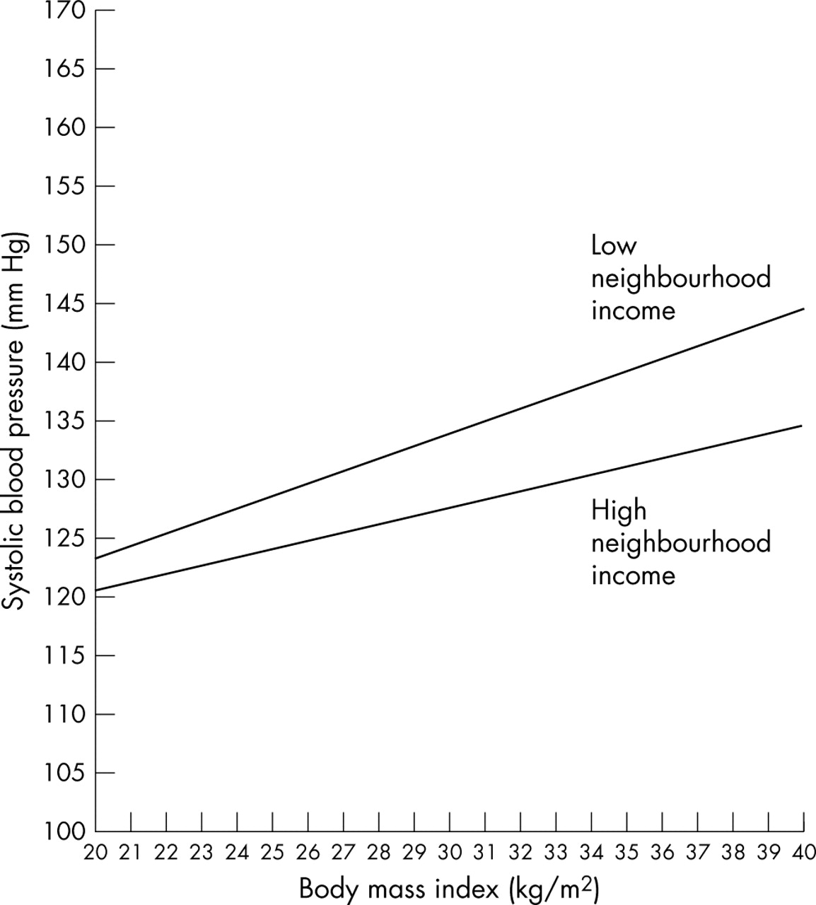
The results presented in table 1 have a direct interpretation. The regression coefficient of the neighbourhood variable shows that over and above individual characteristics—including individual low income—SBP is higher in low income neighbourhoods. We can also see a significant cross level interaction between the effects of neighbourhood low income and individual BMI, so that the increase of SBP with BMI is more intense in low income neighbourhoods. Another interpretation of this interaction is that the difference in SBP between low and high income neighbourhoods is more intense for people with a higher BMI. Figure 1 plots this interaction effect.

Study of random effects (measures of health variation)

In this section we use some general MLRA concepts, such as proportional change in variance (PCV), random slope, variance function, and variance partition coefficient (VPC) that have been presented and discussed in a previous publication.¹³

The neighbourhood disparities, or variance, in SBP persist after adjustment for the individual composition of the neighbourhoods in terms of age, AHD use, BMI, and individual low income. By including the neighbourhood low income variable in model v we can now observe how much of the remaining neighbourhood SBP differences are explained by the level of socioeconomic deprivation in the neighbourhoods.

We have previously explained¹³ that the coefficient of the association between BMI and SBP—the slope—may be allowed to be random at the neighbourhood level. This procedure is called random slope analysis or random cross level interaction analysis, and informs us as to whether the effect of individual BMI on SBP differs from one neighbourhood to another. Because of the existence of a BMI slope variance, the neighbourhood variance becomes a function of BMI. The reader will find more detailed information on this aspect in a previous companion article of this series¹³ and elsewhere.^11,15

In table 1 we see that, taking the between neighbourhood variance of the intercept of model iv⁰ as a reference of comparison, the inclusion of neighbourhood low income in model v explained 22% of the neighbourhood differences in SBP. However, as the neighbourhood variance is a function of BMI, this percentage concerns only the intercept variance, which corresponds to the neighbourhood variance for people with a BMI of 25 kg/m² (that is, when the mean centred BMI is equal to 0). In fact, as the neighbourhood variance is a function of individual BMI, the inclusion of the neighbourhood low income in model v explains a different amount of the neighbourhood variance for people with different BMI values. This phenomenon is illustrated in figure 2A, where we see that the reduction in neighbourhood variance when comparing model v with model iv⁰ is greater for people with higher BMI values. This procedure provides relevant information, showing that causal pathways between the neighbourhood socioeconomic environment and individual SBP may be differentiated for people with a different BMI.

We have previously explained that the VPC is the proportion of the variance in SBP that is located at the neighbourhood level. In the simplest form the VPC corresponds to the intraclass correlation (ICC).¹³ In our case, the VPC is a function of BMI, as both the individual and neighbourhood variances depend on the BMI value.¹³ It is rather intuitive that neighbourhood influences could be more intense on certain groups of individuals than on others. The VPC allows us to operationalise the idea that the clustering of a phenomenon within neighbourhoods—that is, its contextual dimension, may be of different magnitude for people with different characteristics.

We can see in figure 2B that the VPC was reduced for every person, whatever their BMI value, when information on neighbourhood low income was introduced in the model. This reduction in VPC suggests that some part of the contextual phenomenon related to individual SBP was attributable to neighbourhood deprivation. In table 1, the VPC in people with a BMI value of 25 kg/m² was slightly reduced from 0.08 in model iv⁰ to 0.07 in models v and v⁰. However, as the between neighbourhood differences in SBP (that is, variance) depend on individual BMI values, the complete picture as to how VPC changes when the neighbourhood variable is included in the model is presented in figure 2B. Even if the interpretation of the values of the variance function at the extreme of the curve is less reliable because of the lower number of people with extreme BMI values, we realise from this figure that a larger share of the neighbourhood variations in SBP was explained for people with a higher BMI. After taking into account the neighbourhood income level, we still see that the unexplained neighbourhood disparities in SBP (that is, neighbourhood residual variance) remained more important for people with high BMI values than for people with normal BMI.

DISCUSSION

In our hypothetical example we found that individual SBP was partly conditioned by the neighbourhood of residence of the persons. About 8% of the individual SBP differences were attributable to the neighbourhood level, after taking into account differences in the individual composition of the neighbourhoods in terms of age, use of AHD, BMI, and individual low income.

Neighbourhood low income explained a fraction of the SBP disparities, but did not account for all of the individual clustering of SBP within neighbourhoods. In other words, some part of the contextual phenomenon remained unexplained, which was expressed as a residual clustering of individual SBP within neighbourhoods.

Overall, neighbourhood low income increased individual SBP, and modified the association between BMI and SBP. Because of this interaction the effect of neighbourhood low income was especially intense among overweight people, who presented a particularly higher SBP in low than in high income neighbourhoods. A possible explanation for these hypothetical neighbourhood income effects could be that certain contextual factors, such as access to healthcare resources and other facilities, and social norms or social control that may condition blood pressure level by promoting certain lifestyles (for example, physical activity or low salt consumption), may be less favourable in low income neighbourhoods, which may be particularly detrimental for people with high BMI values in these neighbourhoods.

Investigating cross level effects and interactions by means of measures of association and measures of variance

We have seen the existence of a cross level (that is, neighbourhood-individual) effect on SBP. We have investigated this effect by analysing both measures of variance (random slope, variance function, PCV, and VPC)¹³ and measures of association (regression coefficients for the association between neighbourhood low income and SBP and for the interaction between neighbourhood low income and BMI effects).

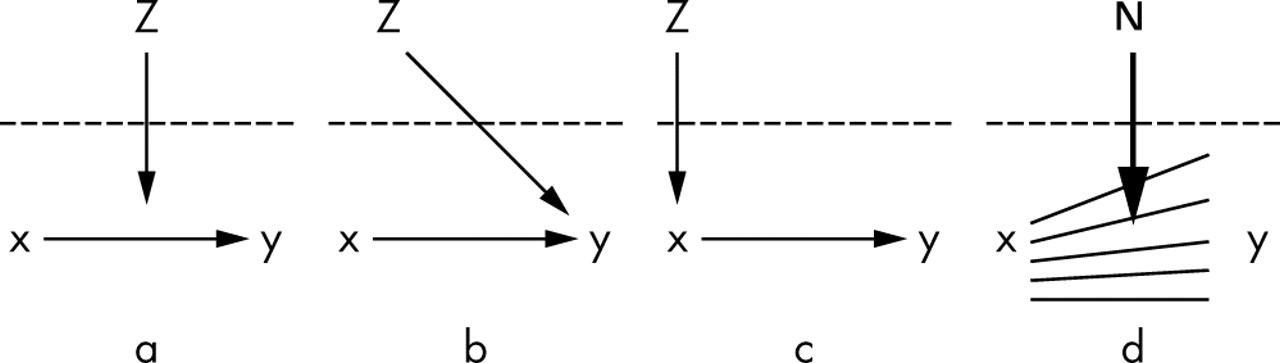
At this point, it is appropriate to briefly mention the differences between fixed and random cross level effects and cross level effect modifications. Following the conventions of Tacq discussed by Snijders⁹ and later adapted by Blakely,¹⁶ there are three important macro-micro relations also termed cross level effects: (a) cross level effect modification (that is, the interaction between neighbourhood low income and BMI effects presented in table 1), (b) direct cross level effect (that is, the direct effect of neighbourhood low income on SBP presented in table 1), and (c) indirect cross level effect. In this last case we could figure out that neighbourhood low income influences SBP by conditioning BMI which, in turn determinates SBP.**

The aforementioned relations are represented in figure 3 where Z is a neighbourhood level variable, x is an individual level variable, and Y is an individual level outcome. These three cross level pathways are commonly investigated by “fixed effect” analysis, that is, by studying measures of association. Relation (a) could be investigated by an interaction term (Z×x) or by dummy variables combining the Z and x categories. Investigating whether relations (b) or (c) exist in the data could be performed by examining whether the regression coefficient of Z changes when adjusting the model for x.

Beyond measures of association (figs 3a to 3c), cross level effect modification analysis can be conducted using random effects (fig 3d). The “random slope” analysis, rather than focusing on the effect of a specific neighbourhood variable Z on Y, examines whether the neighbourhood environment as a whole (N) modifies the association between individual variables (X−Y) without specifying any neighbourhood factors. In our hypothetical example, such cross level effect modification (that is, random slope) was described for the relation between BMI and SBP. The reader will find more detailed information on this aspect in a previous companion article of this series¹³ and elsewhere.^11,15

Including the concept of clustering when interpreting geographical differences in health

We have shown that measuring the clustering of individual health characteristics within neighbourhoods is a concrete way of operationalising the social epidemiological concept of contextual phenomenon.^12,13 Therefore, when it comes to evaluating the importance of considering neighbourhood effects on health, taking into account the size of this contextual phenomenon (that is, the size of clustering as an expression of the contextual dimension of the outcome) may be highly relevant in terms of public health.⁷ Rather than only focusing on aggregated health differences between neighbourhoods or on associations between contextual variables and individual health, the use of measures of clustering informs us as to the relevance of between neighbourhood differences in understanding individual health disparities.

The more the health of the people within a neighbourhood is alike (as compared with the health of people from different neighbourhoods), the more probable it is that the determinants of individual health are directly related to the contextual environment of the neighbourhood, and/or that social processes of geographical segregation are taking place— that is, similar types of individuals choose or are forced to reside in a given neighbourhood.¹²

Figure 4 presents two sets of data showing differences in SBP (on the y axis). The upper sections of the figure (A1 and B1) illustrate the multilevel structure of the data with individual values (represented by a star) nested within neighbourhoods. In the sections A2 and B2, the neighbourhood are ordered by standardised neighbourhood mean income (the x axis). In the lower sections (C and D) the y axis represents the mean blood pressure of each neighbourhood computed by aggregating the individual values in A and B. Figures C and D represent a classic ecological analysis.

Visual inspection of the ecological data (figs 4C and D) shows that the neighbourhood differences in mean blood pressure are of similar magnitude in both sets of data. However, considering the first ecological figure (C), the corresponding multilevel analysis shows that, the clustering of blood pressure values within neighbourhoods is very weak, even before taking into account the neighbourhood income status. In fact, differences between neighbourhoods only account for a very small portion of the total variance in blood pressure (that, the ICC is very low). In the second case (D), the corresponding multilevel analysis shows that the clustering of blood pressure values is very high in the empty model and still very important after taking the neighbourhood income into account as it can be seen in figure B2. In fact, in this extreme example, almost all variability between people is at the neighbourhood level (that, the ICC is very high). We see that the neighbourhood income variable explains a large part of the individual neighbourhood differences in SBP in case B, but only explains a very little share in case A.

Even if ecological observations C and D suggest that there are differences in blood pressure of similar magnitude, multilevel analyses A and B show that the neighbourhood differences over and above individual level differences are very small in C and very important in D.

The purpose of this extreme example is simply to show that an ecological analysis would provide similar information in cases A and B. The multilevel model, on the other hand, provides information on the size of clustering and shows that the two situations are completely different with respect to the relevance of considering neighbourhoods in seeking to understand individual health disparities.

Including the concept of clustering when interpreting the effect of neighbourhood level variables

When studying measures of association (for example, regression coefficients), we aim to obtain information on possible causal relations between neighbourhood characteristics and health. Figure 4 presents a clear association between neighbourhood standardised mean income and blood pressure with a regression coefficient roughly equal to 1.2 mm Hg. This association is similar in A2, B2, C, and D, but the regression coefficient shows nothing of the magnitude of clustering within neighbourhoods that remains after adjustment for the neighbourhood income, which is much larger in B2 than in A2.

Therefore, on the one hand, an association of a given magnitude between a neighbourhood variable and health may explain a large share or alternatively very little of the total individual level variations. And on the other hand, such association may coexist in the model with very small or alternatively very important residual intra-neighbourhood correlations. But the regression coefficient does not provide such information.

The existence of a small ICC in the empty model does not necessarily imply that it is not worth investigating the effects of neighbourhood variables on individual level outcomes.¹⁷ At the same time, however, the existence of an ICC close to 0 does suggest that the context defined by the neighbourhoods is not that important in understanding individual health disparities.

It could be the case that a neighbourhood characteristic, even if significantly associated with the outcome, has almost no importance if it only explains a very small portion of neighbourhood variance. We can also imagine a case in which the neighbourhood variable would explain a large portion of a neighbourhood variance that is itself very small. In that case, explaining a large portion of neighbourhood variance will not make the neighbourhood variable important for public health, as a lot of very little is still very little.¹⁸

By neglecting information on clustering, ecological analyses—as well as the exclusive consideration of measures of association between neighbourhood characteristics and individual health—may lead to the stigmatisation of certain neighbourhoods. Indeed, in ignoring the variability within neighbourhoods, we may assume that the neighbourhood effect applies directly to all the people who live in it, which may lead to inappropriate area stereotypes such as “healthy” or “unhealthy” neighbourhoods. Stigmatisation may lead to neighbourhood blame and discrimination. If inaccurate perceptions of contextual effects are applied to health policy, such policies may be inefficient in reducing inequalities.¹⁹ Therefore, taking into account the magnitude of clustering is especially relevant in the current research on neighbourhood and health. Unfortunately, many published articles do not inform on neighbourhood variance and clustering or simply avoid interpreting it.

Using measures of clustering of individual health status within neighbourhoods, we could evaluate the relative importance of the neighbourhood level for various kinds of outcomes, and may promote neighbourhood level interventions for those health outcomes that are in a greater extent than others determined by the neighbourhood. These considerations are important when attempting to determine the efficacy of focusing intervention on places instead than on people.⁷ For example, if an intervention were to be focused on a given selection of low income neighbourhoods when in fact neighbourhood variation represents only a very small part of the total variation in the health outcome, then many people at risk would be ignored simply because they do not reside in low income neighbourhoods. When the clustering of individual health status within neighbourhoods is small, focusing intervention on specific places may be a rather inefficient strategy.⁷

Combining measures of variation and measures of association is therefore useful in assessing the importance of the neighbourhood environment and its characteristics when seeking an understanding of individual health inequalities.

In this article neighbourhoods were defined as geographical areas. However, multilevel modelling lends itself to a variety of other meanings of community and context including groups defined by cultural rather than by strict geographical administrative areas.²⁰

In this and two previous articles^12,13 we have presented a number of concepts that have not been commonly discussed in multilevel epidemiology despite their importance. Our essay contributes to an understanding of the connection between MLRA and social epidemiological concepts and of the relevance of these concepts for public health, with a special focus on the notion of contextual phenomenon.