Article Text

Abstract
Study objective: Outline the use of the pairwise odds ratio (PWOR) to quantify the extent to which a binary outcome clusters geographically. Quantify the extent to which first experience with cocaine is spatially correlated within US neighbourhoods and cities. Quantify geographical clustering of first experience with cocaine by neighbourhood context.
Design: Estimate the PWOR of incident cocaine experience at two levels (neighbourhood, city) and compare across years. Within years, estimate the PWOR by neighbourhood disadvantage and test for trend.
Setting: US National Household Survey on Drug Abuse.
Participants: Civilian, non-institutionalised household residents of the United States age 12 years and older interviewed in person during 1979, 1988, 1990, 1991, 1992, 1993.
Main results: First experience with cocaine clusters within US neighbourhoods and cities. There is some evidence that the spatial correlation of first experience with cocaine increases with percentage of neighbourhood households living in poverty.
Conclusions: The gradient in spatial correlation of incident cocaine experience by neighbourhood poverty level is consistent with current theories of concentrated disadvantage. The possibility that the direction of the poverty gradient might change over the course of a drug epidemic is discussed.
- space-time clustering
- contextual effects
- multilevel analysis
- PWOR, pairwise odds ratio
- NHSDA, National Household Survey on Drug Abuse
- PSU, primary sampling unit
- SES, socioeconomic status
- CWE, chief wage earner
- ALR, alternating logistic regressions
Statistics from Altmetric.com
- PWOR, pairwise odds ratio
- NHSDA, National Household Survey on Drug Abuse
- PSU, primary sampling unit
- SES, socioeconomic status
- CWE, chief wage earner
- ALR, alternating logistic regressions
Early epidemiological investigations of infectious disease, such as John Snow’s study of cholera, often focused on geographical variation in the occurrence of disease. They compared and contrasted the characteristics of geographical areas in which disease clustered in an effort to uncover aetiological clues. Snow pinpointed cases on maps that led him to discover that geographical context was essential to the spread of cholera in London; the disease clustered in areas served by a water company that drew from the polluted downstream Thames but hardly at all in areas served by its competitor, which drew from an upstream source.1 Recently, there has been a resurgence of interest in the context of health and illness (characteristics of the physical and social environment) as witnessed by the proliferation of “contextual,”2 “multilevel,”3 and “hierarchical”4 studies in the public health and social science literatures.5,6 Some epidemiologists have called for the context of disease, geographical and otherwise, to be incorporated into risk factor epidemiology, the long dominant approach that focuses on associations between individual level risk factors and the risk of illness without necessarily considering the broader context of aetiology.7,8
The contextual approach seeks to open the “black box”9 of risk factor epidemiology by examining whether contexts might place people at risk of risks for illness.10 This study and our previous work11 incorporate geographical clustering, a notion central to early epidemiology, into the contextual approach to epidemiology that has recently become popular. Whereas contextual analyses typically analyse whether geographically defined contexts are associated with the risk of disease, our approach examines whether such contexts are related to the geographical clustering of disease. To demonstrate our approach, we examine the extent to which incident experience with cocaine clusters in relation to the geographical context in which it occurs. Historical distance from the US cocaine epidemic of the 1980s and early 1990s12 coupled with the availability of data from geographically sampled survey data collected during those years make cocaine a worthy candidate for this approach to contextual analysis.
In this paper we address two research questions. Firstly, does incident experience with cocaine cluster geographically and, if so, is the observed spatial correlation an artefact of neighbourhood composition? Secondly, in an attempt to better understand the spatial correlation of cocaine, this paper takes a cue from previous drug research and examines whether the magnitude of clustering of cocaine incidence is associated with neighbourhood disadvantage.13–15
The Office of National Drug Control Policy estimated that the economic costs of illegal drug misuse in the United States (health care costs, loss in productivity, crime related costs, and social welfare costs) rose from $102.2 billion in 1992 to $143.4 billion in 1998 and projected the cost would rise to $160.7 billion in 2000.16 Recent reports indicate that cocaine use, especially in the form of “crack,” is growing rapidly in Europe, most notably in Britain.17–19 Given cocaine’s past cost to and impact on the health of the United States, we believe this study presents a timely examination of the spatial correlation of cocaine incidence and its possible association with neighbourhood disadvantage.
METHODS
This paper reports the results of analyses of public use data from six years of the National Household Survey on Drug Abuse (NHSDA): 1979, 1988, and 1990 to 1993.20–25 The use of multiple years of data facilitates an examination of whether the results replicate. These six years are examined, in part, because their corresponding data were available as NHSDA public use files at the time this study was conceived. More importantly, they were collected during the downward turn in the most recent cocaine epidemic in the United States.12,26 Data from more recent years, after the cocaine epidemic had subsided, might provide misleading results as the underlying factors responsible for the epidemic might have subsided. For example, if the present analyses used data from years in which the incidence of cocaine use had fallen to levels lower than those observed during epidemic years, fewer neighbourhood residents would be starting cocaine use, making it more difficult to detect an association with neighbourhood socioeconomic status.
The NHSDA is a multistage area probability sample of civilian, non-institutionalised household residents of the United States age 12 years and older. It was first conducted in 1971, then periodically during the 1970s and 1980s, and has been conducted annually since 1990. Before the 1991 survey, only the 48 contiguous states were sampled; Alaska and Hawaii were included beginning with the 1991 survey. The primary sampling units (PSUs) randomly selected in the first stage of sampling were standard metropolitan statistical areas, counties, groups of counties and independent cities, or portions of counties, or other well defined geographical units; for ease of discussion, PSUs will hereinafter be referred to as “cities,” the lay geographical term to which they most closely correspond. The 1990 survey oversampled the Washington, DC metropolitan area; the 1991–1993 surveys added oversamples of metropolitan Chicago, Denver, Los Angeles, Miami, and New York City. “Segments” within cities were selected in the second stage of sampling. Segments were defined using aggregations of census blocks and enumeration districts that contained a maximum of 1000 and a minimum of 40 (in 1988) to 90 (in 1993) occupied housing units according to the 1980 census or, in the case of the 1992 and 1993 surveys, the 1990 census. For ease of discussion, segments will hereinafter be referred to as their closest lay equivalent—“neighbourhoods.” Housing units (hereinafter referred to as “households”) within neighbourhoods were selected in the third stage of sampling. The fourth and final stage of sampling entailed selecting zero, one or two respondents from individual households. Complete details of the survey design and sampling procedures can be found in official NHSDA publications. Once respondents were identified, they were recruited into the study according to guidelines approved by an Institutional Review Board. Respondents who agreed to participate answered some interview questions by responding to questions read aloud to them by an interviewer who recorded their oral answers. Respondents answered sensitive questions such as those regarding drug use by reading them from an answer sheet on which they also marked their own replies, which remained unknown to the interviewer. The interview response rate ranged from 77% in 1988 to 84% in 1991.27–32
The NHSDA interview contained modules that include standardised questions about use, opportunity to use, and perceived harm of tobacco, alcohol and other drugs. It also contained a module of questions about demographic characteristics of respondents and their families. Beginning with the 1988 survey, respondents were instructed that all questions about cocaine should be interpreted to include both the powder form of cocaine and crack cocaine unless a question asked specifically about crack cocaine. Accordingly, this study examines both forms of cocaine.
The inclusion of multiple respondents from a household might tend to inflate estimates of geographical clustering when using simpler statistical models. To expedite statistical computations, a single respondent was randomly selected from within those households in which more than one interview was conducted. Furthermore, to estimate the extent to which incident cocaine experience clusters, subjects who were not “at risk” for the respective outcomes had to be removed from the samples. The samples used for this study were therefore smaller than the total sample sizes on the NHSDA public use files.
Variables
This paper examines two outcomes that reflect incident experience with cocaine. Two binary (yes/no) outcomes were constructed from responses to the following two questions30: (1) “About how old were you when you first had a chance to try cocaine, in any form, if you had wanted to?”; (2) “About how old were you the first time you actually used cocaine, in any form, even once?” The two outcomes will be referred to herein as first had opportunity and first used cocaine, respectively.
If neighbourhoods and cities differ in terms of their composition with respect to factors associated with these outcomes, it is possible that estimates of geographical clustering could be artefacts of these differences. For this reason, seven categorical sociodemographic covariates associated with cocaine use33 are incorporated into all of the models reported herein in an effort to examine whether their statistical adjustment might attenuate the estimates of geographical clustering of the outcomes. These seven categorical covariates are: age, race, hispanic ethnicity, sex, marital status, employment status, and educational attainment.
Two additional individual level categorical covariates were also included in the analyses for the purposes of adjustment. People from the same socioeconomic status (SES) tend to cluster their residences in self selected neighbourhoods.34 Because this paper examines whether cocaine outcomes cluster based on geographical area of residence, it is therefore necessary to adjust for SES. We use the combination of educational attainment and occupation to measure SES.35 Because adolescents were included in the sample, we measure occupation of chief wage earner (CWE) in household, which breaks the Census Bureau’s 16 occupational groups into six categories.36 Two additional categories were added to accommodate respondents who: (a) reported their households had no CWE or that the household CWE does not work; (b) did not report the occupation of their household CWE.
The other individual level covariate included for the purposes of adjustment is residential mobility. This binary covariate (moved/did not move) was constructed from responses to the following question: “How many times in the past five years have you moved?”23 Beyond its reported association with the cocaine outcomes,33 residential mobility is used in an attempt to adjust for the presence of selection effects. Cocaine users might cluster in particular neighbourhoods by way of two different processes or some combination thereof. People with a proclivity to use or have opportunity to use cocaine might migrate to certain locations, thereby selecting the neighbourhoods in which they cluster. Selection effects might also occur when persons who are not likely to use or have opportunity to use cocaine selectively migrate from particular neighbourhoods, leaving behind a cluster of persons who do have these characteristics.37 The analyses reported in this paper attempt to adjust for selection effects by incorporating this measure of residential mobility as a covariate in our analyses.
Finally, of the few neighbourhood level measures of neighbourhood disadvantage available on the NHSDA public use data files examined herein, we chose the only one that allowed for examination of a gradient in within neighbourhood clustering. This measure of disadvantage, percentage of households in poverty, is derived from 1990 census data. It is included only on the 1992 and 1993 NHSDA public use files and appears as a six category variable (quintiles plus a missing category) to prevent possible disclosure of any respondent’s identity.
Statistical methods
The extent to which the binary cocaine outcomes co-occur within geographical areas can be quantified using alternating logistic regressions (ALR), a recently developed statistical method.38 The ALR method uses first order generalised estimating equations39 to regress a binary outcome on covariates while simultaneously estimating a pairwise odds ratio (PWOR) by regressing each binary response in a geographical area on others from the same geographical area. To address the first research question, we use ALR to quantify the extent to which first experience with cocaine clusters within US cities and neighbourhoods. To quantify geographical clustering in this way necessitates the estimation of nested models because neighbourhoods are nested within cities. To address the second research question, we use ALR with a contextual pairwise model to quantify the extent to which incident experience with cocaine clusters within neighbourhoods by level of neighbourhood disadvantage (see appendix).
RESULTS
Table 1 displays the number of cities, neighbourhoods and respondents in each of the six NHSDA samples after removal of respondents not “at risk” of the respective outcome (that is, those who had their first opportunity to use cocaine, or first used cocaine, more than five years ago). The two incidence measures declined steadily between 1979 and 1993: First had opportunity drops from 15.6% of respondents in 1979 to 8.0% of the 1993 sample. First used cocaine falls from 8.4% of respondents in 1979 to 2.8% of the 1993 sample. (Because of space limitations, cross tabulations of the outcomes by the nine sociodemographic covariates under consideration are not presented here but are available upon request.)
Figure 1 illustrates that first had opportunity and first used cocaine cluster within neighbourhoods; it displays within neighbourhood PWORs and their 95% confidence limits for six years of data. For each outcome, five of the six PWORs are greater than unity. The extent to which first had opportunity clusters within neighbourhoods ranges from 1.20 (95% CI = 1.00 to 1.44) in 1990 to 1.69 (95% CI = 1.35 to 2.12) in 1993. (The unadjusted counterpart PWORs (not depicted) are 1.20 in 1990 and 1.88 in 1993.) The estimates for first used cocaine range from 1.30 (95% CI = 1.01 to 1.66) in 1990 to 1.92 (95% CI = 1.29 to 2.86) in 1979. (The unadjusted counterpart PWORs (not depicted) are 1.42 in 1990 and 2.38 in 1979.)
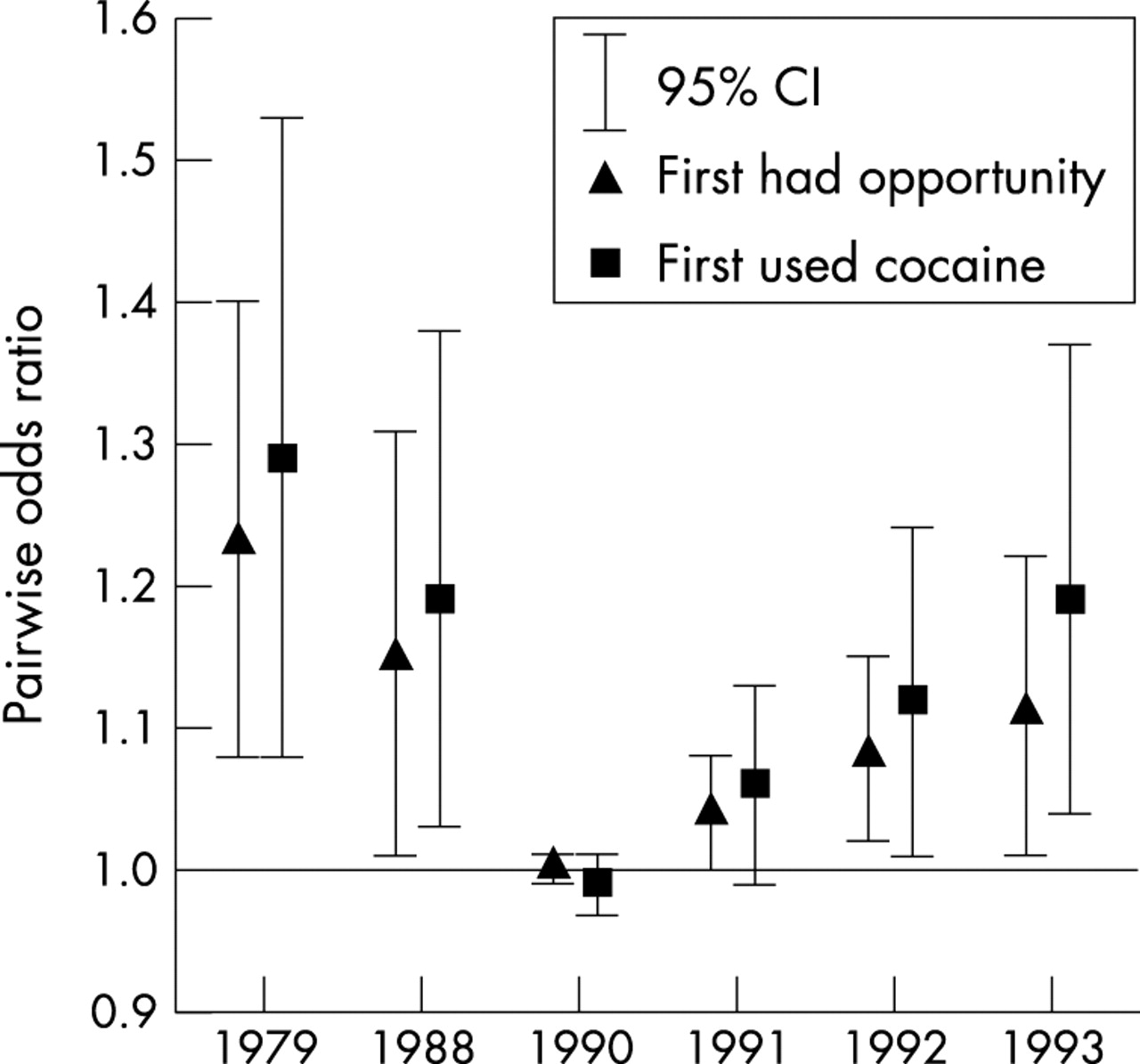
Figure 2 illustrates both outcomes cluster within cities. It displays the within city PWORs, and their 95% confidence limits, from the same models used to estimate the within neighbourhood PWORs in figure 1. Recall that the within city PWOR quantifies the residual clustering within cities once clustering within neighbourhoods has been taken into account. For each outcome, four of the six PWORs are greater than unity. The extent to which first had opportunity clusters within cities ranges from 1.00 (95% CI = 0.99 to 1.01) in 1990 to 1.23 (95% CI = 1.08 to 1.40) in 1979. (The unadjusted counterpart PWORs (not depicted) are 1.01 in 1990 and 1.22 in 1979.) The estimates for first used cocaine range from 0.99 (95% CI = 0.97 to 1.01) in 1990 to 1.29 (95% CI = 1.08 to 1.53) in 1979. (The unadjusted counterpart PWORs (not depicted) are 1.00 in 1990 and 1.32 in 1979.) For both outcomes, within city clustering decreases from 1979 to a minimum in 1990 and increases thereafter.
Figure 3 illustrates within neighbourhood clustering of first had opportunity increases with neighbourhood poverty level in 1992 (z = 2.97) but not in 1993 (z = 0.68). In 1992, within neighbourhood clustering ranges from 1.16 (95% CI = 0.91 to 1.47) in the least impoverished neighbourhoods to 1.94 (95% CI = 1.54 to 2.46) in the most impoverished. (The unadjusted counterpart PWORs (not depicted) are 1.24 and 2.17, respectively.) Between the two extremes of poverty, within neighbourhood clustering of first opportunity increases with increasing poverty rate. In 1993, clustering ranges from 1.54 (95% CI = 1.17 to 2.01) in the least impoverished neighbourhoods to 1.79 (95% CI = 1.45 to 2.22) in the most impoverished. (The unadjusted counterpart PWORs (not depicted) are 1.93 and 1.80, respectively.) In 1993, a gradient effect is precluded by a high degree of clustering in neighbourhoods with 2.66% to 5.12% poverty (PWOR = 1.75; 95% CI = 1.07 to 2.86).
Figure 4 illustrates within neighbourhood clustering of first used cocaine increases with neighbourhood poverty level in 1992 (at z = 1.92) but not in 1993 (z = 0.55). In 1992, first use is least clustered in the least impoverished neighbourhoods (PWOR = 0.67; 95% CI = 0.39 to 1.14) and most clustered in the most impoverished neighbourhoods (PWOR = 2.08; 95% CI = 1.34 to 3.24). (The unadjusted counterpart PWORs (not depicted) are 0.62 and 2.40, respectively.) Between the two extremes of poverty, within neighbourhood clustering of first use increases with increasing poverty rate. In 1993, the estimates do not display a gradient; first cocaine use is least clustered in neighbourhoods with 5.13% to 9.02% poverty (PWOR = 1.05; 95% CI = 0.60 to 1.82) and most clustered in neighbourhoods with 9.03% to 16.15% poverty (PWOR = 1.65; 95% CI = 0.99 to 2.75). (The unadjusted counterpart PWORs (not depicted) are 1.19 and 1.63, respectively.)
DISCUSSION
This study outlines the use of the pairwise odds ratio to measure a different kind of contextual effect: the extent to which a binary outcome clusters geographically. It presents the first quantitative estimates of the magnitude of spatial correlation of incident experience with cocaine at two levels of analysis, neighbourhoods and cities, and by level of neighbourhood disadvantage. The findings are replicated using six separate years of survey data collected during the downward turn in the most recent US cocaine epidemic. First opportunity to use cocaine co-occurs within neighbourhoods from 1.2 to 1.7 times more often than one would expect if it were distributed randomly across neighbourhoods, and first use of cocaine co-occurs from 1.3 to 1.9 times more often. Once within neighbourhood concentration has been taken into account, there is evidence of modest residual clustering of incident experience with cocaine within cities. Furthermore, there is some evidence that spatial correlation of first opportunity to use cocaine and first cocaine use increase with neighbourhood poverty level. Neighbourhood composition with respect to age, race/ethnicity, sex, socioeconomic status, and residential mobility does not explain the spatial correlation of incident experience with cocaine within neighbourhoods in general, or within poorer neighbourhoods in particular.
One possible explanation for geographical clustering of cocaine incidence within neighbourhoods is “contagion”: a contextual effect in which the probability that a person will develop a disease outcome is dependent upon the degree to which others in the community already have the outcome.7,40 In other words, the rate at which unaffected people become affected (that is, incidence) depends upon the prevalence rate of disease within a group.41 Despite its connotation, the contagion effect can describe non-infectious diseases and the adoption of health behaviours within groups.7,42 For example, current drug users might encourage use among non-users in the community and thereby transmit the behaviour and increase the incidence and prevalence rates.42 In other words, beliefs and behaviours are transmitted from neighbour to neighbour.43,44 DeAlarcon reported how heroin use spread in such a fashion among residents of a London suburb in the 1960s.45 Hughes and Crawford used this model in an attempt to intervene in Chicago’s heroin epidemic of the early 1970s.46
Another possible explanation for clustering of first cocaine experience within neighbourhoods involves “selection” processes, selective in-migration and/or out-migration from neighbourhoods. This study adjusted for selection effects by incorporating a measure of residential mobility as a covariate. However, it is important to distinguish selection processes which produce poverty from the social processes by which neighbourhood contexts produce spatially clustered outcomes.47 Elsewhere, we found no evidence of differences in geographical clustering of cocaine when it was estimated separately by the residential mobility status of respondents.48
Key points
-
The pairwise odds ratio (PWOR) can be used to quantify the extent to which a binary outcome clusters geographically. The PWOR can be estimated by the statistical method of alternating logistic regressions.
-
First opportunity to use cocaine and first use of cocaine cluster within US neighbourhoods to an extent that is not explained by neighbourhood composition.
-
Once spatial correlation within neighbourhoods of these two incident outcomes has been accounted for, there is modest residual spatial correlation within US cities.
-
There is some evidence that the spatial correlation of these outcomes within neighbourhoods increases with neighbourhood poverty level.
Limitations
A thorough interpretation of the estimates presented herein necessitates a brief discussion of several limitations of the data and methods used. The NHSDA data are self reported and their validity are affected by respondents’ truthfulness and memory, and possibly by socially desirable responding with respect to the behaviour in question.49 Although NHSDA procedures encourage honesty and recall, the data are likely to contain some measurement error.
The use of NHSDA “segments” as a proxy for “neighbourhoods” presents some conceptual difficulties. The ideal measurement of neighbourhoods would not rely solely on geographical boundaries but would instead capture the social dimensions of neighbourhoods, such as cohesion and shared institutions and values, which have been called “the ultimate mechanisms through which neighbourhood effects can be transmitted.”47 The small size of NHSDA segments (maximum of 1000 occupied housing units) makes them a less problematic stand-in for neighbourhoods than such commonly used constructs as census tracts, but their small size is no guarantee that they somehow embody the interpersonal connections one wishes to quantify when speaking of “neighbourhood effects.”44 The same conceptual problem exists when equating NHSDA primary sampling units with “cities.”
Future research
One facet of the utility of examining whether within neighbourhood clustering of first experience with cocaine (or other drug use or other inherently social health problems) varies by neighbourhood context rests in its potential for identifying types of neighbourhoods to target for preventive intervention. However, it is perhaps too broad a generalisation, or too simplistic, to suggest that preventive interventions should be targeted to impoverished neighbourhoods. The cross sectional survey data examined here cannot speak to the underlying mechanisms that might give rise to the observed spatial correlation of first experience with cocaine within neighbourhoods. Future research should apply and evaluate strategies designed to uncover the social mechanisms that drive the geographical clustering of cocaine and other drug use, such as those proposed by Frohlich et al50 and Macintyre et al.51
Several historical examples drawn from the 20th century experience in the US suggest that the use of cocaine, or “club drugs” such as MDMA (“ecstasy”), may occur more often in the upper socioeconomic strata when they first gain popularity but then drift downward as the epidemic gains momentum. Hence, the “tipping point” described by Crane52 might actually characterise the end stages of epidemics of social problems. It is possible that in the earlier stages of an epidemic the poverty gradient in clustering of first cocaine experience might be inverted, such that clustering is highest in affluent neighbourhoods and lowest in impoverished neighbourhoods. This speculation cannot be investigated with respect to the recent US cocaine epidemic because the requisite data are not available. The early warning signs of a cocaine epidemic in Britain17–19 suggest a potential opportunity to examine the plausibility of this hypothesis.
Inclusion of more specific survey questions regarding experience with cocaine and other drugs would be useful. For example, survey questions that ask respondents whether they shared or sold drugs to their neighbours could help evaluate the plausibility of the contagion interpretation of geographical clustering of incident drug outcomes. Furthermore, the NHSDA asks when first experience with cocaine and other drugs occurred, but not where; knowing whether it occurred at home, school, work, or outside the neighbourhood would be essential in any attempt to discern the mechanisms driving geographical clustering.
Finally, although we conducted a preliminary evaluation,48 more definitive research into the potential effect of incorporating sampling weights into the estimation of geographical clustering is necessary. Similarly, it is unknown whether survey designs that include geographically defined oversamples, such as the 1991–1993 NHSDA six city oversample, affect estimates of spatial correlation.
Conclusions
The results of this study concur with recent theories of concentrated disadvantage. William Julius Wilson demonstrated that the social transformation of inner city neighbourhoods during the 1970s and 1980s resulted in an increasing concentration of poverty.53 This concentration of the most disadvantaged segments of the population produces what he calls “concentration effects”: “the constraints and opportunities associated with living in a neighbourhood in which the population is overwhelmingly socially disadvantaged—constraints and opportunities that include the kinds of ecological niches that the residents of these communities occupy in terms of access to jobs, availability of marriageable partners, and exposure to conventional role models” (page 144). He also describes the growth of the inner city illicit drug industry as a concentration effect, which, in turn, can increase rates of drug use in high poverty neighbourhoods.54 Work inspired by Wilson suggests that both poverty and affluence are highly geographically concentrated in the United States.34,55 Furthermore, Massey discussed increasing rates of drug use as a potential ramification of the concentration of affluence and poverty.55
Policy implications
-
Geographical clustering of the earliest stages of involvement with cocaine suggests prevention efforts might be more effective if they were geographically targeted.
-
In the later stages of a cocaine epidemic, the effect of prevention efforts might be increased if they were targeted to disadvantaged neighbourhoods.
-
Based on previous experience with cocaine and other drugs, it is possible that in the earlier stages of an epidemic the poverty gradient in clustering of first experience with a drug might be inverted, such that clustering is highest in affluent neighbourhoods and lowest in impoverished neighbourhoods. The early warning signs of a cocaine epidemic in Britain suggest a potential opportunity to examine the plausibility of this hypothesis.
One of the more intriguing findings in this study, which might be added to the body of evidence on concentration effects, involves the interplay between the geographical clustering of first experience with cocaine and neighbourhood disadvantage. Because the results encompass both first opportunity to use cocaine and first use of cocaine, one can be more certain that the spatial correlation of first opportunity to use, one of the earliest points in the progression through drug involvement, is engendered by concentrated disadvantage or associated conditions in the neighbourhood environment. It is not easy to imagine how clusters of opportunity to try cocaine could cause neighbourhood residents to become more impoverished in any direct manner. Rather, it seems more likely that concentrated neighbourhood disadvantage itself, or characteristics associated with it such as a lack of social capital56 or collective efficacy,57 might give rise to conditions that favour the occurrence of a first experience with cocaine.
APPENDIX
Whereas an ordinary odds ratio is defined in terms of subjects, the PWOR is defined in terms of all possible pairs of subjects. It can be defined using a standard two by two table:
| 2nd subject in pair has outcome? | |||
|---|---|---|---|
| Yes | No | ||
| 1st subject in pair has outcome? | Yes | A | B |
| No | C | D | |
Two by two table
Note that the cells of the above table refer to pairs of subjects, not single subjects, with respect to their values on an outcome of interest. Pairs concordant on the outcome are counted in cells A and D. Discordant pairs are evenly split between cells B and C; the PWOR therefore considers combinations, but not permutations, of the outcome among pairs of subjects.
The PWOR is calculated like an ordinary odds ratio by taking the cross product ratio (AD/BC).58 As its name implies, the PWOR is the ratio of two odds. The numerator of the ratio represents the odds that one respondent in the pair has the outcome when the other respondent has the outcome (A/C). The denominator represents the odds that one respondent has the outcome when the other does not have the outcome (B/D).
The PWOR measures the extent to which an outcome clusters among respondents within pre-defined geographical areas and can range from zero to infinity. A value of one is consistent with an absence of spatial correlation of the outcome. A PWOR greater than one indicates how many times more often the outcome co-occurs among respondents compared with what one would expect if the outcome occurred randomly. The PWOR, however, is not merely a function of prevalence or incidence rates. Areas with a lower rate of disease than others could have a higher degree of clustering. For example, although typhoid rates are higher in less industrialised nations where it is endemic, it is more geographically clustered in industrialised nations because it occurs as sporadic localised outbreaks. A PWOR indicating no geographical clustering, on the other hand, does not indicate the rate of disease is the same for all areas.
ALTERNATING LOGISTIC REGRESSIONS (ALR)
The utility of the PWOR becomes more apparent when it is used to compare different groups of subjects. The scenario above considers all possible pairs of subjects without reference to any intrinsic differences between them. The method of alternating logistic regressions can estimate the PWOR across categories of subjects defined in various ways. The design of the NHSDA allows one to partition subjects on the basis of geographical units. One way this study defines subjects is according their geographical residence—neighbourhoods and cities. Another way is by the poverty level of the neighbourhood in which a subject resides.
I NESTED MODEL
Let Yijk denote the presence or absence of a cocaine outcome for the kth respondent in the jth neighbourhood in the ith city. The log PWOR regression model, or “pairwise” model, is written:

where Zijkℓm = 1 if j = ℓ (that is, respondents k and m reside in the same neighbourhood) and Zijkℓm = 0 otherwise. For example, in the case of pair (Y111, Y112),

because the pair (k = 1 and k = 2) reside in the same city (i = 1) and neighbourhood (j = 1). However, in the case of pair (Y121, Y113),

because the pair (k = 1 and k = 3) reside in the same city (i = 1) but different neighbourhoods (j = 2 and j = 1, respectively). It follows that exp(α0) is the within city PWOR and exp(α0+α1) is the within neighbourhood PWOR.
The within neighbourhood PWOR estimates the odds of a cocaine outcome for a respondent from a neighbourhood where a randomly chosen respondent from the same neighbourhood has the same outcome relative to the odds if that respondent does not have the same outcome.58 It quantifies, in other words, how often a cocaine outcome co-occurs within neighbourhoods relative to what one would expect if it were distributed randomly. The within city PWOR estimates the odds of a cocaine outcome for a respondent from a city where another randomly chosen respondent from the same city but different neighbourhood has the same outcome relative to the odds if the randomly chosen respondent does not have the same outcome. In other words, it quantifies how often a cocaine outcome co-occurs within cities relative to what one would expect if it were distributed randomly, regardless of any non-randomness within neighbourhoods. Because it considers pairs of respondents from the same city but different neighbourhoods, the within city PWOR reflects the residual clustering of the outcome within cities after accounting for clustering within neighbourhoods.
Let X*ijk denote the value of covariate X* for the kth respondent in the jth neighbourhood in the ith city. The ALR model simultaneously estimates a GEE logistic regression of a cocaine outcome on covariates:

As in a conventional logistic regression, exp(β) is interpreted as an odds ratio. The inclusion of a covariate that describes respondents and is associated with the outcome will increase or decrease the within city or within neighbourhood PWOR, depending on the direction of the correlation of the covariate within cities and/or neighbourhoods.58
The ALR algorithm alternates between the logistic model of the outcome and the log odds ratio regression of the pairwise associations until convergence.38 The impact of adding covariates to the logistic model can be gauged by comparing the unadjusted and adjusted estimates of the PWOR.59 The inclusion of covariates in the logistic model can be interpreted as adjusting the within neighbourhood PWOR for the composition of neighbourhoods with respect to those covariates. The ALR method is implemented as an S-Plus (Insightful Corporation S-Plus, version 3.4) function that estimates the regression coefficients and covariance matrices from the pairwise and logistic models (Carey VJ, ALR, version 4D, http://www.biostat.harvard.edu/~carey/old_public_html/index.ssoff.html).
As the ALR method has not yet been augmented to incorporate sampling weights, we evaluated their impact on the estimated PWORs by partitioning the NHSDA samples based on quartile of sampling weight and re-estimating selected models. The estimates did not vary in a consistent manner with quartile of sampling weight.48
II Contextual model
Let Yijk be a binary variable that represents the presence or absence of a cocaine outcome for the kth respondent in the ith neighbourhood of type j. To examine clustering within neighbourhoods of different types, we write the pairwise model as:

where Zijkℓm = 1 if j = ℓ (k & m reside in the same neighbourhood, which is of type j) and Zijkℓm = 0 otherwise. It follows that exp(α0) is the PWOR for the reference type of neighbourhood and exp(α0+αj) is the PWOR within neighbourhood type j. The logistic model is specified in the same manner as in the nested model. For each outcome and year, we use the contextual ALR model to estimate within neighbourhood clustering by neighbourhood poverty level and test the PWORs for trend.
Incident cocaine outcomes from six years of the National Household Survey on Drug Abuse
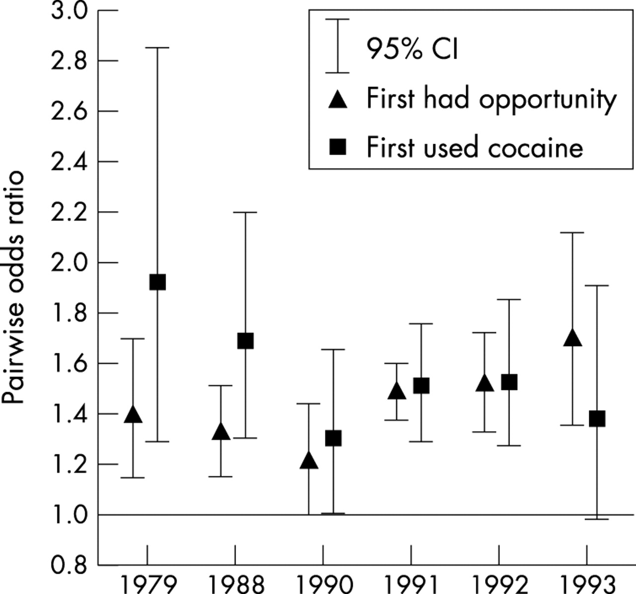
Geographical clustering within US neighbourhoods of two incident cocaine outcomes.

Residual geographical clustering within US cities of two incident cocaine outcomes.

First had opportunity to use cocaine during past five years: within neighbourhood clustering by neighbourhood poverty level.

First used cocaine during past five years: within neighbourhood clustering by neighbourhood poverty level.
Acknowledgments
This research was made possible by research grants R01 DA09592 and R01 DA09897 and training grant T32 DA07292, all from the National Institute on Drug Abuse, and by a service fellowship from the Office of Applied Studies at the Substance Abuse and Mental Health Services Administration. Vincent J Carey and Scott L Zeger provided much appreciated statistical consultation. We are very grateful to the anonymous reviewers whose comments considerably sharpened the conceptual approach of this paper. Thanks to Pete Shelley for the title idea (“decide for yourself; listen to others”).