Article Text

Abstract
Study objective: (1) To provide a didactic and conceptual (rather than mathematical) link between multilevel regression analysis (MLRA) and social epidemiological concepts. (2) To develop an epidemiological vision of MLRA focused on measures of health variation and clustering of individual health status within areas, which is useful to operationalise the notion of “contextual phenomenon”. The paper shows how to investigate (1) whether there is clustering within neighbourhoods, (2) to which extent neighbourhood level differences are explained by the individual composition of the neighbourhoods, (3) whether the contextual phenomenon differs in magnitude for different groups of people, and whether neighbourhood context modifies individual level associations, and (4) whether variations in health status are dependent on individual level characteristics.
Design and participants: Simulated data are used on systolic blood pressure (SBP), age, body mass index (BMI), and antihypertensive medication (AHM) ascribed to 25 000 subjects in 39 neighbourhoods of an imaginary city. Rather than assessing neighbourhood variables, the paper concentrated on SBP variance between individuals and neighbourhoods as a function of individual BMI.
Results: The variance partition coefficient (VPC) showed that clustering of SBP within neighbourhoods was greater for people with a higher BMI. The composition of the neighbourhoods with respect to age, AHM use, and BMI explained about one fourth of the neighbourhood differences in SBP. Neighbourhood context modified the individual level association between BMI and SBP. Individual level differences in SBP within neighbourhoods were larger for people with a higher BMI.
Conclusions: Statistical measures of multilevel variations can effectively quantify contextual effects in different groups of people, which is a relevant issue for understanding health inequalities.
- MLRA, multilevel regression analysis
- SBP, systolic blood pressure
- AHM, antihypertensive medication
- VPC, variance partition coefficient
- BMI, body mass index
- multilevel analysis
- blood pressure
- neighbourhoods
- social epidemiology
Statistics from Altmetric.com
- MLRA, multilevel regression analysis
- SBP, systolic blood pressure
- AHM, antihypertensive medication
- VPC, variance partition coefficient
- BMI, body mass index
Persons with similar characteristics may have different health experiences according to whether they live in one neighbourhood or in another, and people living in the same neighbourhood tend to experience a similar health status. This is in part because people in the same neighbourhood are subject to common contextual influences. This contextual phenomenon that expresses itself as clustering of individual health status within neighbourhoods is a core notion in social epidemiology.1–5 Despite this rationale, the study of clustering in social epidemiology is insufficiently valued. Indeed, current multilevel epidemiology mostly investigates associations between contextual factors and individual health, using multilevel techniques to obtain accurate statistical estimates for measures of association such as regression coefficients. It is necessary to use procedures like multilevel regression analysis (MLRA) that consider the connection of the outcome health variable among people from the same area (clustering) to obtain unbiased standard errors for regression parameters.6–8 However, as we have emphasised elsewhere,4 the clustering of individual health within neighbourhoods far from being a statistical nuisance, remains a key topic of investigation in social epidemiology, as it conveys essential information to our understanding of contextual phenomena.4,7,9,10
This paper is an expansion of that idea.4 It seeks to express an epidemiological vision of multilevel analysis that focuses on clustering and other measures of health variation to enlarge our knowledge of the distribution and determinants of a population’s health status. We discuss the concept of variance partition coefficient (VPC) as illustrative of the relative importance of the context as a function of individual characteristics. The clustering of individual health within areas, however, may reflect the varying composition of neighbourhoods in terms of individual characteristics, rather than true contextual effects. Therefore, we also show how to determine the extent to which neighbourhood disparities in health may change after taking into account differences in the individual composition of the neighbourhoods. Finally, we illustrate that the neighbourhood context may modify the association between individual characteristics and health. The epidemiological approach to MLRA used here is of relevance in public health for understanding both the patterns and determinants of geographical and social disparities in health.
Our objective was to provide a didactic and conceptual (rather than mathematical) link between MLRA and social epidemiological concepts. Readers who wish a more formal or alternative statistical explanation may consult the referenced studies on multilevel analysis published elsewhere.6–8,11–13
This report is based on hypothetical data regarding systolic blood pressure (SBP). Its conclusions, therefore, must not be taken as empirical evidence.
POPULATION AND METHODS
The study model population and variables
The population of our study model consists of 25 000 people 35 to 64 years old, living in the 39 neighbourhoods of a hypothetical city. It presents a clear multilevel structure with people (level 1) nested within neighbourhoods (level 2). The individual outcome variable is SBP. For didactic reasons and to keep the model as simple as possible, only three individual variables were included: (1) age in years, (2) body mass index (BMI) in kg/m2 (both of the aforementioned variables were centred on their overall mean of 49 years and 25 kg/m2, respectively), and (3) whether any antihypertensive medication (AHM) was used. No neighbourhood variable was investigated in this article. For simplicity, age and BMI effects were assumed to be linear.
Our study model was adapted from an actual empirical investigation analysing countries rather than neighbourhoods that was published elsewhere.14
MLRA
Using MLRA we investigate (1) whether there is significant clustering within neighbourhoods (model 1), (2) to which extent neighbourhood level differences are explained by the individual composition of the neighbourhoods (model 2), (3) whether the contextual phenomenon differs in magnitude for different groups of people, and whether neighbourhood context modifies individual level associations (model 3), and (4) whether variations in health status are dependent on individual level characteristics (model 4)
The “empty” MLRA model (model 1)
The empty MLRA model is more extensively discussed in a companion paper15 and elsewhere.6–8,16 It does not include explanatory variables but only estimates the city SBP mean and the neighbourhood level and individual level differences in SBP. In this model, the variations in SBP between neighbourhoods are assumed to be of similar magnitude for every person. In using this model, we simply aim to identify a possible contextual phenomenon that can be quantified by clustering of SBP within neighbourhoods.15
The MLRA model with individual variables (model 2)
This model expands the empty model (model 1) by including the individual variables age, BMI, and use of AHM as fixed effects. “Fixed effects” and “random effects” are expressions that are often used in MLRA. Essentially, fixed effects are used to model averages (for example, means or regression coefficients), whereas random effects are used to model differences (for example, neighbourhood variance).17
In equation 1 we present model 2 using non-conventional notation that will be better understood by readers not trained to read formal statistical notation. An individual level variable is shown by subscript I, and neighbourhood information shown by N. Readers who wish a more formal statistical notation are referred elsewhere.6–8,12

SBPI = SBP of a given individual (I) in a given neighbourhood.
Fixed effects
SBPC = SBP in people not on AHM and with average age and BMI (which correspond with a value of 0 as these variables are centred), and living in a neighbourhood with a shrunken residual equal to 015
β1 = regression coefficient of the association between age and SBP
β2 = regression coefficient of the association between BMI and SBP
β3 = regression coefficient of the association between AHM and SBP
Random effects
EN = neighbourhood shrunken residual15
EI = individual residual
In MLRA models, it is assumed that the residuals are normally distributed and that the individual level residuals and the neighbourhood level residuals are independent. In MLRA, both people and neighbourhoods are assumed to be randomly sampled from a population of individuals and a population of neighbourhoods.
As in simple regression analysis, the regression coefficients of the individual variables in MLRA describe the association between the individual level variables and SBP.* The regression coefficients in table 1 show that SBP increases with age and BMI, as expected. Use of AHM is associated with higher SBP, reflecting that the condition underlying this treatment is simply hypertension.
Hypothetical multilevel regression analysis of systolic blood pressure (SBP) (mm Hg) in 25 000 people aged 35 to 64 from 39 neighbourhoods of a city
The presence of neighbourhood and individual residuals in the model reflects that SBP varies at both levels. The variance is a summary of the differences, and including individual variables in the statistical models allows us to obtain values of variances that are adjusted for age, BMI, and AHM use. The adjusted total SBP variance between people in the city (VTotal) can be partitioned into a variance between neighbourhoods (VN) and a variance between people within neighbourhoods (VI) as explained more extensively in an earlier related paper.15
In both models 1 and 2, the neighbourhood SBP differences correspond to the neighbourhood variance of the intercept. In model 2, the intercept is the value of the outcome variable SBP when the explanatory variables are equal to zero. In that case, the expected intercept value is equal to SBPC + EN, which is the neighbourhood SBP estimated mean for 49 year old people with a BMI of 25 kg/m2 (as continuous individual level variables are centred on their means) without AHM treatment. However, the neighbourhood variance in model 2 is, in fact, the same for all the individuals, whatever their individual characteristics. This aspect can be seen graphically in figure 1, and can also be interpreted in saying that the relation between BMI and SBP is considered to be the same in all neighbourhoods. Using the coefficient estimates from table 1, the expected value of SBP increases by 0.88 mm Hg for every unit of increase in BMI, regardless of whether the person resides in a neighbourhood or another.
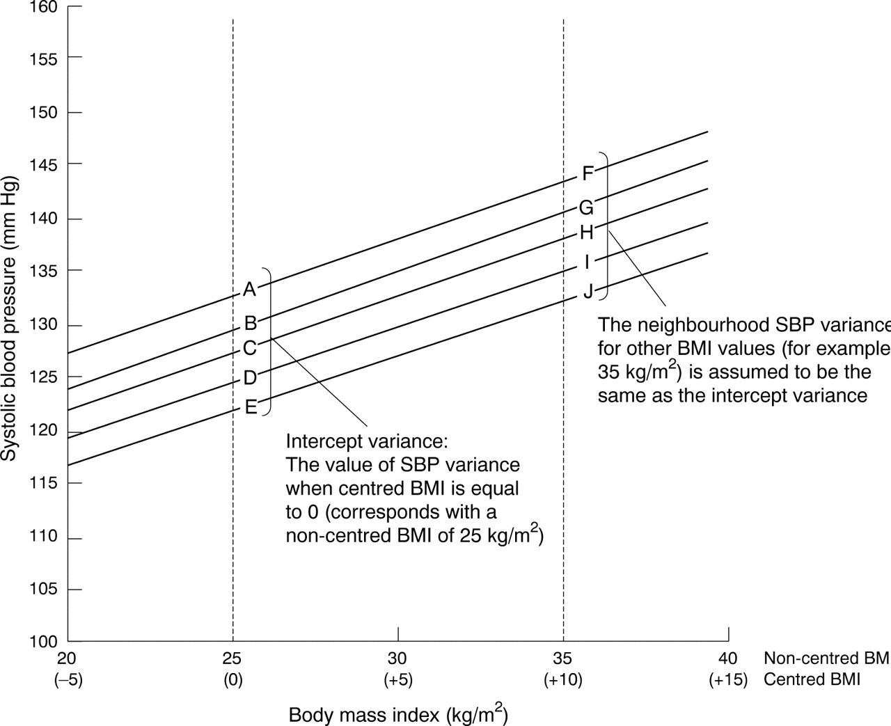
The regression lines represent the association between body mass index (BMI) and systolic blood pressure (SBP) in five hypothetical neighbourhoods of an imaginary city. Note that the lines are parallel. The neighbourhood lines have a different intercept but a similar slope. Therefore, differences between the neighbourhoods are constant for every BMI value (that is, the differences between points A, B, C, D, and E, and between F, G, H, I, and J on the vertical dotted lines at BMI values 25 and 35 kg/m2 are of similar magnitude). Note that the BMI value of 25 kg/m2 corresponds to the mean BMI for the city and also corresponds to the value 0 for the centred BMI, as BMI is centred on its mean in the regression models.
Proportional change in variance at different levels
Neighbourhood differences in mean SBP may be attributable to contextual influences or to differences in the individual composition of neighbourhoods in terms of age, BMI, AHM use, and other individual characteristics not considered in our didactic study model. By adjusting for individual characteristics in model 2, we take into account some part of the compositional differences and explain some of the neighbourhood variance detected in the empty model (model 1).† The equation for the proportional change in neighbourhood variance‡ (PCVN) is:

where VN-1 is the neighbourhood variance in the empty model and VN-2 is the neighbourhood variance in the model including individual characteristics. For example, comparing model 1 with model 2, PCVN is equal to (36.2–27.6)/36.2. We conclude that 24% of the neighbourhood SBP variance in the empty model was attributable to the three compositional factors considered.
This equation can be adapted to calculate the proportional change of variance at the individual (I) level (PCVI), as individual SBP variance within neighbourhoods will also be explained by differences in age, BMI, and AHM use.

In table 1, we see that 29% of the individual SBP differences (that is, within neighbourhoods variance) in the empty model was attributable to differences in age, BMI, and use of AHM.
The intraclass correlation
Using the values of the adjusted variance at both levels we calculated the adjusted intraclass correlation (ICCAdj). We have explained the concept of ICC in a previous paper on this topic.15 This measure is of relevance, as it quantifies clustering of individual SBP within neighbourhoods and, therefore, can be used to operationalise the concept of contextual phenomena.4,15

The ICCAdj is the proportion of total variance in SBP that remains at the neighbourhood level after taking into account the individual composition of the neighbourhoods in terms of age, BMI, and AHM use.§ Table 1 shows that about 8% (ICC equal to 0.08) of the individual residual differences in SBP were related to the neighbourhood level and might be attributable to contextual factors.¶
Even if compositional confounding remains in the data,16,17 model 2 suggests that the neighbourhood context conditions a common level of blood pressure over and above individual age, BMI, and AHM use.
Note that in models 1 and 2, we have calculated a single ICC value for the whole city, with the assumption that all people are influenced by the neighbourhood context in an equivalent extent.
The multilevel regression model with individual variables and random slopes (model 3)
In model 3 (equation 5) we relinquish the idea that the magnitude of the association between BMI and SBP is similar in all neighbourhoods. Rather, we assume that the effect of BMI on SBP may vary depending on the neighbourhood context. For example, it is possible that contextual factors in some neighbourhoods have a higher impact on overweight people than in people with normal BMI. In model 3, therefore, we extend model 2 by allowing the regression coefficient of BMI to vary randomly at the neighbourhood level:

β2C = mean regression coefficient of the association between BMI and SBP in the city
EN-BMI = shrunken difference between β2C and the specific regression coefficient in a given neighbourhood
EN-c = shrunken difference between the city SBP mean and the neighbourhood SBP mean for individuals with a BMI equal to 25. See our previous related paper for an explanation of the concept of shrunken residual.15
Neighbourhood mean and slope differences (intercept and slope variances between neighbourhoods)
In model 3, aside from the neighbourhood differences in mean SBP (that is, the intercept variance VN-c), each neighbourhood has its own regression coefficient for the association between BMI and SBP, and each neighbourhood coefficient deviates from the city mean regression coefficient (β2C) by a residual amount (EN-BMI). This slope variability is measured by the slope variance (VN-BMI). In MLRA, this procedure is called random slope analysis or random cross level interaction analysis. It suggests that the neighbourhood context modifies the individual level association between BMI and SBP. A graphic illustration of random slopes is presented in figure 2, where it may be seen that the slope of the association between BMI and SBP is steeper in some neighbourhoods than in others.

The regression lines represent the association between BMI and SBP in five hypothetical neighbourhoods. The lines are not parallel, as we do not only have variations in the intercept but also in the slope of the association. The lines are not only separated by an amount corresponding with the different neighbourhood SBP means (that is, intercepts), but are also separated by varying amounts for different BMI values. As the slopes of the regression lines are different, the differences between the neighbourhoods are not constant for every BMI value, as in figure 1 (the differences between points A, B, C, D, and E, and between F, G, H, I, and J on the vertical dotted lines at BMI values 25 and 35 kg/m2 are not equal). The individual level variance within neighbourhoods is represented as triangles around the regression lines. The triangles represent a non-constant individual level SBP variance. The individual level SBP variance within neighbourhoods increases with BMI.
Correlation between the intercept and slope residuals
It may occur that in those neighbourhoods with a high mean SBP (a high intercept residual value), the slope of the association between BMI and SBP is steeper (the residual value for the slope is higher). We can express this connection as a coefficient of correlation according to equation 6:

where the variances (VN-c, VN-BMI) and the covariance between the intercept and slope residuals (Cov(N-c)•(N-BMI)) are parameters that are directly estimated by the multilevel model.
Table 1 shows that the slope variance (VN-BMI) is 0.11, the intercept variance (VN-c) is 27.6, and the covariance between the intercept and the slope residuals (Cov(N-c)•(N-BMI)) is 0.93. Using the estimates and applying equation 6 we find that the correlation between the intercept and the slope is equal to 0.53. Figure 3 illustrates this correlation and suggests that on average BMI has a stronger impact on SBP (that is, the slope of the association is steeper) in neighbourhoods with a higher mean level of SBP (that is, a higher value of the intercept).

There is a correlation between the residuals associated with the intercept and the residuals associated with the slope of the association between BMI and SBP. The figure shows that this correlation is positive, which can be interpreted as follows: in neighbourhoods with a higher mean level of SBP (a higher value of the intercept), BMI has a stronger impact on SBP (the slope of the association is steeper). According to the parameters estimated in model 3 (table 1), the correlation between the intercept and the slope is equal to 0.53.
Beyond the interest of examining whether an individual level association varies between neighbourhoods, a relevant reason to consider random slopes is to examine whether neighbourhood differences in SBP have a different magnitude among people with different characteristics. Figures 2 and 4 give a graphic illustration of this concept. In our study model the neighbourhood variance now depends on individual BMI: it is no longer a single value as in models 1 and 2, but a function of BMI. The figure 2 shows that there is more neighbourhood variability in SBP among those who have a higher BMI.

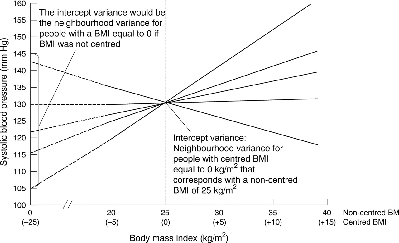
The figure represents a case in which the intercept variance is zero (on the dotted line at BMI equal to 25 kg/m2). However, because of random slopes, even if the variance is zero for the intercept, the variance is very large for people with a BMI of 35 kg/m2 (the dotted line at BMI equal to 35 kg/m2). Centring the variables on the city BMI mean ensures that the neighbourhood intercept variance can be directly interpreted. This figure shows that, if the BMI was not centred on its mean of 25 kg/m2, the intercept variance would correspond to people with a BMI equal to 0 kg/m2, who obviously do not exist. The regression lines have been prolonged as dotted lines to represent the intercept variance if the BMI was not centred.
Considering neighbourhood variance as a function of individual level variables (equation 7) yields improved information on the shape of neighbourhood differences. The neighbourhood variance function and its confidence intervals are directly calculable by available software.13 The interested readers will find another practical example and a more formal statistical explanation elsewhere.18,19

Table 1 provides the values of the intercept variance, the slope variance, and the covariance between the intercept and the slope needed in equation 7. The full shape of the neighbourhood differences as a function of BMI is presented in figure 5A. These neighbourhood differences seem to be larger for overweight people, reflecting the fact that the neighbourhood context modifies the individual association between BMI and SBP.

Neighbourhood and individual variances (A) and variance partition coefficient (VPC) (B) are shown as a function of individual BMI. Both the neighbourhood level and the individual level variances increase with BMI. We provide the 95% confidence intervals of these functions. Note that the predicted variance is more uncertain for the extreme values of BMI. The neighbourhood context seems to influence individual SBP. However, this contextual influence differs in magnitude between people with a different BMI. Neighbourhood differences in SBP were greater for obese people (VPC around 12%–14%) than for people with normal BMI (VPC = 8%).
Note that in models 1 and 2 with random intercept only, the neighbourhood level variance is assumed to be the same for all people. We can, therefore, compare the intercept variance in models 1 and 2 with any value of the variance function VN in model 3.
It is important to note that the assumption that neighbourhood differences are the same for all people may conceal significant contextual effects that pertain to specific groups of people. In such cases, the neighbourhood heterogeneity can only be properly identified when random slopes are taken into account and the variance is calculated as a function of individual characteristics. Figure 4 contains a hypothetical situation in which the neighbourhood context strongly modifies the individual association between BMI and SBP. In figure 4, the neighbourhood differences (intercept variance) is close to null; but for people whose centred BMI is over and under zero, the neighbourhood variance is very large and suggests that the context has apparent importance.
The multilevel regression model with individual variables, random slopes, and non-constant individual variance (model 4)
We can hypothesise that within each neighbourhood individual SBP differences are higher among those who are overweight than among people of normal BMI. In statistical terms this phenomenon is called individual level heteroscedasticity, meaning that the individual level variance in SBP is not constant along BMI. This is shown in figure 2, where triangles surrounding the regression lines show that individual level SBP variations within neighbourhoods increase with BMI. Absence of heteroscedasticity is a precondition for doing correct regression analysis. We can use MLRA to model non-constant individual level variance and obtain both relevant epidemiological information and correct regression estimates.
Model 4 (equation 8) is similar to model 3 (equation 5) but includes an additional individual level residual, which is related to BMI (EI-BMI).

As every group of people with a particular BMI value has a specific individual level SBP variance, the individual level variance also becomes a function of BMI.
In equation 9 we provide a very simple expression of this function; more details on the equation may be found elsewere.19 As in the case of neighbourhood variance, this variance function is directly calculable with available softwares.13

where VI-c is the individual variance related to the intercept, V I -BMI is the individual level variance related to BMI, and Cov(I-c)•(I-BMI) is the covariance between the two sets of individual level residuals.
Modelling of individual variance may not only significantly improve the fit of the statistical model and the validity of the regression estimates but also provides useful information when it comes to understanding SBP inequalities among individuals and neighbourhoods.
Variance functions and the variance partition coefficient (VPC)
In contrast with models 1 and 2, the neighbourhood level and individual level SBP variances in models 3 and 4 are no longer represented by one simple value. The complete picture of the variances in our study model is presented in figure 5A that has been obtained using equations 7 and 9. Figure 5A shows that both individual level and neighbourhood level variances increase considerably with BMI.
As suggested earlier, contextual influences may be stronger for certain groups of people such as overweight people, and less important for people with normal BMI. To quantify this aspect, we must examine how differences in SBP are partitioned between the individual level and the neighbourhood level for different BMI values. Rather than one ICC, we calculate a VPC that is function of the BMI (VPCBMI),6,19 using the neighbourhood level (VN ) and individual level (VI) variance functions of equations 7 and 9.

As shown in table 1, the VPC in model 3 is about 0.08 in people with a BMI of 25 kg/m2, which means that 8% of the variations for these people were at the neighbourhood level. The VPC as a function of BMI is presented in figure 5B and shows that the VPC was equal to 0.14 (14%) for people with a BMI of 40 kg/m2. Even if the values of variance function at the extremes of the curve are less reliable, the neighbourhood context seems to play a more relevant part for people with high BMI.
DISCUSSION
We have attempted, on the basis of hypothetical data, to illustrate the investigation of a contextual phenomenon that expressed itself as a clustering of individual SBP within neighbourhoods. According to our findings, this contextual phenomenon was—at least partly—independent of the composition of the neighbourhoods, and has a different impact on people with a different BMI. Indeed, as people living in the same neighbourhood share common contextual influences, they tend to experience a similar SBP level. For example, you might hypothesise that neighbourhood disparities in access and quality of hypertension care may condition neighbourhood specific degrees of blood pressure control over and above individual differences.
In our study model we found that the neighbourhood context influenced overweight people to a greater extent than normal weight people. Possible explanations could be that physicians in some neighbourhoods treat overweight people with hypertension more intensively than physicians in other neighbourhoods, or that interventions directed to factors that affect SBP (for example, physical activity or low salt diet) are more efficient in certain neighbourhoods.
The association between BMI and SBP was stronger in neighbourhoods with a higher level of SBP (the correlation between the intercept and the slope was equal to 0.53). To explain this pattern, it could be hypothesised that obese people tend to present higher SBP in neighbourhoods with less successful blood pressure control strategies (that is, with higher SBP means).
Therefore, as a whole, our study emphasises a vision of MLRA that focuses on measures of health variation for understanding the distribution of health status in the population.4 In describing complex patterns of variation, MLRA provides useful information for analysis of cross level (for example, neighbourhood-individual) causal pathways.
Despite their relevance, some of the concepts presented here have not been widely discussed in the literature on multilevel analysis. The analysis of patterns of variance, which has been undervalued in many previous investigations, contributes to our understanding of the distribution and determinants of geographical, social, and individual disparities in health status.
Our didactic presentation shows the link between the statistical concepts of MLRA and the social epidemiological notion of contextual phenomenon and permits a better assessment of the interest of MLRA in social medicine and public health research.
Footnotes
-
↵* In MLRA, however, the mathematical interpretation of the regression coefficients is not exactly the same as in the standard non-multilevel model not adjusted for the neighbourhood residuals. Interested readers can obtain an extended explanation elsewhere.8
-
↵† Note however that individual characteristics may be in the causal pathway between neighbourhood characteristics and individual differences in SBP, so including individual characteristics in the model may result in understating the contribution of contextual influences to SBP. The interpretation of the PCV therefore depends on the individual variables included in the model, and on their hypothesised role (that is, confounding role, mediating role).
-
↵‡ The proportional change in variance is often referred to as “explained variance”. However, the addition of individual variables in the model may increase the second level variance. Indeed, in cases in which the neighbourhood differences are hidden by their individual composition, the total variance may decrease but the neighbourhood component of the variance increase. Therefore, “proportional change in the variance” is a more appropriate term than “explained variance”.
-
↵§ Note however that individual variables like BMI may be in the causal pathway between neighbourhood characteristics and individual differences in SBP, so including BMI in the model may result in understating the contribution of contextual influences to SBP. The interpretation of the IPC therefore depends on the individual variables included in the model, and on their hypothesised role (that is, confounding role, mediating role).
-
↵¶ Observe that the ICC was the same in the empty model and in the model with individual variables. The inclusion of individual level predictors reduced the individual and neighbourhood level variances by the same amount proportionally, what was reflected in the IPC.
-
Funding: this study is supported by grants (principal investigator Juan Merlo) from the Swedish Council for Working Life and Social Research) (number 2002-054 and number 2003-0580), and from the Swedish Research Council (number 2004-6155)
-
Conflicts of interest: none.