Article Text

Abstract
Study objective: To evaluate methods for calculating life expectancy in small areas, for example, English electoral wards.
Design: The Monte Carlo method was used to simulate the distribution of life expectancy (and its standard error) estimates for 10 alternative life table models. The models were combinations of Chiang or Silcocks methodology, 5 or 10 year age intervals, and a final age interval of 85+, 90+, or 95+.
Setting: A hypothetical small area experiencing the population age structure and age specific mortality rates of English men 1998–2000.
Participants: Routine mortality and population statistics for England.
Main results: Silcocks and Chiang based models gave similar estimates of life expectancy and its standard error. For all models, life expectancy was increasingly overestimated as the simulated population size decreased. The degree of overestimation depended largely on the final age interval chosen. Life expectancy estimates of small populations are normally distributed. The standard error estimates are normally distributed for large populations but become increasingly skewed as the population size decreases. Substitution methods to compensate for the effect of zero death counts on the standard error estimate did not improve the estimate.
Conclusions: It is recommended that a population years at risk of 5000 is a reasonable point above which life expectancy calculations can be performed with reasonable confidence. Implications are discussed. Within the UK, the Chiang methodology and a five year life table to 85+ is recommended, with no adjustments to age specific death counts of zero.
- life expectancy
- small areas
- Monte Carlo method
Statistics from Altmetric.com
In 2001 the UK government described life expectancy (LE) as the best summary measure of health outcome.1 A national inequality target aims to reduce the gap between the areas with the lowest LE at birth and the population as a whole by at least 10% over the next decade.2 Consequently, there is now a great deal of interest in understanding the methods used for calculating LE in small areas, particularly electoral wards (average population 6000).
Since William Farr produced national English life tables in the 1840s,3 and contrasted the health status of three English districts, progress towards producing LE in small areas has been slow. In the 1970s, Gardner and Donnan used life table techniques to compare LE among hospital regions within England and Wales.4 Analysing mortality data for the period 1981 to 1992, Charlton described variations in LE between different types of local authorities and different groups of electoral wards.5 Raleigh and Kiri, using data for the period 1984–94, calculated LE for district health authorities.6 In 1995, Williams et al argued that the populations of health districts were likely to conceal wide internal variations in mortality, leading to important health differences being overlooked. Abridged population life tables were calculated for electoral wards within the London borough of Croydon, showing a variation of 5.4 years between the highest and lowest wards,7 and life expectancies for 27 electoral wards were presented in the annual public health report.8
In 2001 Griffiths et al examined geographical variation in LE in the UK, producing abridged life tables for local authorities, but excluded from their analysis the Isle of Scilly (population 2100) and the City of London (population 7100) “as there are too few deaths there in a three-year period to make analysis meaningful”.9 The authors argued that numbers at ward level were too small to allow meaningful LE calculations to be done. Silcocks et al used a population of 256 000 to investigate the sampling distribution and usefulness of LE at health district level and below.10
In England the Office for National Statistics publishes life expectancies for local authority and health authority areas 11 using the methodology described by Chiang.12,13 Recently, the Trent Public Health Observatory has produced LE calculations at ward level using the Silcocks’ methodology.14
Two important questions arise. Firstly, what is the preferred methodology for doing small area LE? Secondly, what is the smallest size of population years at risk for which robust LE calculations can be performed?
STUDY AIMS
The objective of our research is to evaluate the methods for calculating LE in small areas such as English electoral wards. The four principal aims are to:
1 Compare the Chiang and Silcocks methodologies
Both Chiang and Silcocks LE methodologies are based on the construction of a current life table. The two methodologies differ in the assumptions used to convert the observed age specific mortality rates into the age specific survival probabilities. While Chiang uses a linear method that assumes deaths are distributed evenly through an age interval, Silcocks assumes that the mortality rate is constant throughout an age interval, resulting in the number of survivors decreasing exponentially.
2 Investigate the effect of different age intervals
Life tables may be complete, where the mortality experience is broken down by single years of life, or abridged, in which larger age intervals are used, usually of 5 or 10 years. For small areas, practicality dictates that abridged life tables must be used. The affect of different age intervals on the estimates of LE was investigated, examining 5 year compared with 10 year age intervals and different final age intervals (85+, 90+, 95+).
3 Examine the precision of LE estimates
In England, confidence intervals are not commonly quoted for LE estimates, even for sub-national areas such as local authorities. Both Chiang and Silcocks provide a formula for calculating the standard error but, again, their assumptions differ. Chiang assumes that observed age specific deaths are binomially distributed, while Silcocks assumes a Poisson distribution. In age intervals where death is a rare event the two distributions are approximately equivalent. However, for some age intervals the magnitude of the mortality rate is such that death cannot be considered as a rare event and there is some debate as to which distribution is the most appropriate to use.15 Each methodology was tested, using deaths simulated from the distribution upon which that methodology is based.
The final difference between the two methods is the variance term for the final age interval. Chiang assumes that as the probability of survival in this interval is, by definition, zero, the associated variance is also zero. Silcocks et al argue that for the final age interval the LE is dependent, not on the probability of survival, but on the mean length of survival, and included a term for the variance based upon this assumption. Here, it is considered that the Silcocks argument is valid, and the additional variance term has been included within the Chiang methodology. This is reflected in the results by the label Chiang (adjusted). Note that the adjustment affects the estimate of the standard error only and not the LE estimate itself.
4 Investigate the effect of zero death counts on standard error estimates
Another problem associated with small populations is the occurrence of zero deaths in an age interval. Silcocks noted that a zero count gives an estimate of zero for the sample variance of the age interval, which is an underestimate of the true variation. This results in an underestimation in the total life table variance, and, therefore, of the LE standard error. The greater the number of zero death counts, the greater the underestimation of the standard error. Silcocks suggested two possible values, 0.693 and 3.0, as possible substitutes for zero counts. These values are the Poisson means for which the probability of observing zero deaths is 50% and 5% respectively.
A zero death count is particularly important in the final age interval. If there are zero observed deaths, the death rate (Mω) is zero, and the hypothetical cohort surviving to the start of the final age interval will have an infinite mean length of survival (1/Mω), giving an infinite LE. In such instances an alternative rate must be used, such as the appropriate national or regional rate or the (weighted) average rate of the surrounding areas. In this study, the equivalent death rate for England was used.
STUDY METHODOLOGY
Monte Carlo simulations were performed, for a hypothetical population of varying size, to describe the distribution of the LE estimate and its standard error estimate. The population age structure and the underlying age specific mortality rates of the population were set to those of English males 1998–2000,16,17 allowing comparisons to reference LE figures published by the Government Actuaries Department.18
A single simulation consisted of 10 000 repetitions. For each repetition, the underlying age specific mortality rate and population for each of the age intervals of the life table model being tested were used to generate a random count of deaths from a known probability distribution. These counts were inserted into a life table to generate an estimate of LE and its standard error. The results of the repetitions produced distributions of LE and standard error estimates from which inferences could be made.
Key points
-
All the life table models tested increasingly overestimated life expectancy as the population size decreased.
-
The overestimation was greatest for life tables using 95+ as the final age interval and least for those using 85+.
-
Life expectancy estimates are normally distributed even for small populations.
-
The standard error estimates are normally distributed for large populations, but become increasingly skewed as the population size decreases.
-
Substitution methods to compensate for the effect of age specific death counts of zero on the standard error estimate were found not to improve the estimate.
Simulations were performed for each methodology, for 5 and 10 year age intervals, to the final age intervals of 85+/90+/95+, or 85+/95+, respectively. The first years of life were broken down into the age groups under 1 and 1–4 years. Simulations using Chiang assumed the binomial distribution for generating random counts of death, while those using Silcocks assumed the Poisson distribution. Simulations were repeated for the hypothetical population years at risk: 500; 1000; 5000; 10 000; 25 000, and 50 000.
To investigate the potential problem caused by zero deaths in an age interval, a count of such occurrences was recorded for each repetition. Simulations were also repeated for each of the following substitutions for zero deaths: none; values 0.693, 3 or the expected number of deaths in both the LE and standard error calculation; and values 0.693, 3 or the expected number of deaths in the standard error calculation only.
A Microsoft Excel application was developed to perform the simulations, and the results were exported to SPSS for statistical analysis.
A reference LE and standard error, for each abridged life table model, was calculated using the underlying mortality rates directly. An additional unabridged reference LE was calculated for each methodology using the underlying mortality rates in an unabridged life table.
RESULTS
Table 1 shows the reference LE for each of the abridged models, the unabridged life table and Government Actuaries Department figures for comparison. The reference LE is independent of the population size as it is calculated from the exact underlying rates.
Reference and simulated life expectancy (LE) by methodology and population size; assuming the population age structure and mortality rates of English men 1998–2000
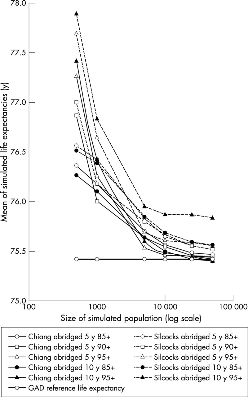
The abridged life tables using Chiang produced slightly better approximations to the GAD reference figure than those using Silcocks. For all the alternative age interval models, the Silcocks’ methodology produced higher expectancies than did the Chiang methodology. For both methodologies five year age intervals resulted in better estimates than 10 year intervals.
Table 1 shows the mean of simulated life expectancies for each life table model, for population years at risk ranging from 500 to 50000. Each mean is the average of the 10 000 life expectancies generated by the repetitions for that particular model and population size.
It was expected that the mean simulated life expectancies would be independent of the population size but this is not the case (fig 1). For all life table models, smaller population sizes gave higher estimates of the LE. As the population size increases, the mean simulated life expectancies approach their corresponding reference LE. For populations greater than 5000, the choice of methodology is the most important factor in estimating LE, with all Chiang models giving better approximations than any of the Silcocks’ models. In populations of 500, the most important factor is choice of the final age interval, with models using the 85+ end point giving the best approximations to the GAD reference figure. This suggested that a significant proportion, if not all, of the “drift” in the mean simulated LE for smaller populations might be found in the final age interval.

Mean of simulated life expectancy estimates by life table methodolgy and size of simulated population; assuming the population age structure and mortality rates of English males 1998–2000.
Both Chiang and Silcocks estimate the mean survival within the final age interval by 1/Mω, where Mω is the mortality rate of the final age interval. The left hand side of figure 2 shows the distribution of 10 000 simulated Mω for the 85+ age interval of a Chiang model, for population sizes of 50 000, 10 000, and 5000. The distribution of the simulated rates is a weighted binomial (being the binomially distributed death counts divided by the 85+ population). As the population size increases, this distribution tends towards the normal and the standard deviation decreases. The mean of the distribution, which is an estimate of the underlying mortality rate, is independent of the population size.

Distribution of simulated mortality rate and mean survival time in the 85+ age interval by population size; assuming the population age structure and mortality rates of English men 1998–2000.
The right hand side of figure 2 shows what happens when these simulated rates Mω are transformed to give the simulated mean survival of the final age interval, 1/Mω. The right hand tail becomes stretched, and as population size decreases, the skewing of the transformed survival time distribution increases, shifting the distribution mean further and further to the right. This results in an overestimate of the underlying survival time, and consequently the LE.
Using 90+ or 95+ as the final age interval, as compared with 85+, generally results in larger drifts in the LE estimate for small populations. This is because the populations in these age intervals are smaller, resulting in greater skewing of the transformed survival times.
Similar effects can be expected in the other, finite, age intervals where the years of life lived during the interval is related to the probability of dying (Chiang) or probability of survival (Silcocks), both of which are transformations of the mortality rate Mi.
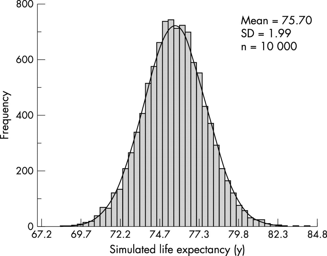
Silcocks demonstrated that LE estimates are normally distributed. The results of this project confirm this finding, showing that it remains true even for population sizes of 5000 (fig 3). This is an important observation, as the normal approximation method used to calculate 95% confidence intervals for the LE (that is, 95%CI = ±1.96 × SE) remains valid for small populations.

Distribution of simulated life expectancy for a population of 5000; using the Chiang methodology with a five year abridged life table to 85+ and assuming the population age structure and mortality rates of English men 1998–2000.
Table 2 shows the standard error of LE estimates by population size. Three measures of the standard error are given: the first is the reference, calculated using the exact underlying mortality rates; the second is the “observed”, found by measuring the standard deviation of the simulated distribution of LE estimates (for example, figure 3); and the third is the “mean estimated”, that is, the mean of the simulated distribution of standard error estimates. We are interested in the mean estimated standard error. By describing the distribution of these simulated standard errors we may infer how the standard error estimate of real data will behave.
Reference and simulated standard error of life expectancy (LE) by methodology and population size; assuming the population age structure and mortality rates of English men 1998–2000
The table shows that the standard error increases as the population size decreases. For the given age structure, and underlying mortality rates, the standard error increases from approximately 0.6 years for 50 000 population, to 1.4 years for 10 000 population, and 4.3 years for 1000 population. The Chiang (adjusted) and Silcocks methodologies give similar estimates of the standard error. For populations over 1000, the width of the age intervals and the choice of the final age interval have little effect.
Examination of the distributions of standard error estimates showed that for population sizes down to 10 000 the distribution closely follows the normal. For smaller populations, however, the distribution becomes increasingly skewed (fig 4). The width of the distribution indicates the precision of the standard error estimate. For the population size of 5000, the mean estimate of standard error is 1.96 years, but its associated standard deviation is relatively large at 0.40 years.

Distribution of simulated life expectancy standard error by population size; using the Chiang methodology with a five year abridged life table to 85+ and assuming the population age structure and mortality rates of English men 1998–2000.
A further feature of table 2 is the good agreement of the mean estimated standard error to the reference and observed standard errors. While the reference and observed figures are unaffected by the problem of zero death counts, it was expected that the mean estimated figure would increasingly underestimate the true standard error as the population size decreased and zero deaths counts became more frequent. This occurs to a small degree for a population size of 500, but it was anticipated that the underestimation would be greater, and evident at larger population sizes.
We examined the mean estimated standard error by the frequency of the zero death counts, and demonstrated that repetitions with a higher frequency of zero deaths give lower estimates of LE standard error (fig 5). The effect holds for both methodologies, and various age structures, and remains evident, although to a lesser degree, at a population size of 50 000. The most plausible reason that this effect does not manifest itself in the overall mean estimate is that a mechanism, similar to that which causes the overestimation of the LE itself, causes an overestimation of the standard error, counterbalancing the underestimation caused by the occurrence of zero deaths.

Simulated life expectancy standard error versus the occurrence of zero death counts in the simulated life table, by population size; using the Chiang methodology with a five year abridged life table to 85+ and assuming the population age structure and mortality rates of English men 1998–2000.
Given this unexpected robustness in standard error estimates, it was unsurprising that none of the substitution methods tested produced better estimates (table 3).
Effect on simulated life expectancy (LE) and standard error of substituting for zero deaths by substitution method; population of 5000, using the Chiang methodology with a five year abridged life table to 85+ and assuming the population age structure and mortality rates of English men, 1998–2000
DISCUSSION
This is the first study, of which the authors are aware, to systematically evaluate the application of standard LE methodologies to populations of small areas.
LEs estimated using the Chiang and the Silcocks methodologies showed good agreement. However, for use in calculating small area LEs in England the Chiang methodology is recommended. It gave the better estimates when compared with the GAD reference and is consistent with the methodology used by ONS for larger populations. For estimating the LE standard error, we propose that the Chiang methodology be adjusted to include a term for the variance associated with the final age band, as suggested by Silcocks.
The choice of the final age interval is important. LE becomes increasingly overestimated as the population size diminishes. This effect is greatest with a final age interval of 95+, and least with a final age interval of 85+. We propose that for small populations 85+ is used as the final age interval. For other age bands the choice between 5 or 10 year age intervals is more arbitrary, and depends upon the availability of accurate denominator information. We recommend that, within England, five year age bands are used to retain consistency with ONS methods.
The increasing number of zero death counts within the life tables of small populations did not affect estimates of LE standard error to the degree anticipated. Methods of correcting standard error estimates by substituting zero death counts did not give better results than the simple, uncorrected method. We recommend, therefore, that no substitutions are made for zero death counts, except where this occurs in the final age interval. Such a count, if not substituted, would lead to an infinite LE. In such instances, an appropriate national, regional, or locally derived, age specific mortality rate should be used.
Estimates of LE are normally distributed even for very small populations. As population size decreases the standard error increases and it becomes increasingly difficult to show statistically significant differences between areas. A population years at risk of 5000, with the same age structure and mortality rates as England men in 1998–2000, has a LE standard error of approximately two years, giving a 95% confidence interval of ±4 years. For a population of 1000 this interval rises to over ±8 years. This compares with a difference of approximately 8.5 years between the highest and lowest English local authority male life expectancies in the period 1998–2000.11 For smaller populations this differential will be greater but it is clear that for English populations smaller than around 5000 only those at the extremes of the range will show statistical significance.
The estimate of the standard error is subject to sampling variation, which increases as the population size falls. The 95% confidence interval of the estimated LE standard error, quoted above for a population of 5000, is itself a relatively large ±0.8 years. A further problem with estimating standard error of small populations is that its distribution becomes increasingly skewed.
In summary, when applying standard life expectancy methodologies to increasingly small populations the problems of overestimation of the LE, increasingly wide confidence intervals and increasingly poor estimation of its standard error must be carefully considered. For small areas in England, we suggest that a population years at risk of 5000 is a reasonable point above which LE calculations can be performed with confidence. For many areas it will be necessary to aggregate data either geographically or over time, particularly if sex specific life expectancies are required. Aggregating over time is simpler but raises issues over the precision of population years at risk estimates. Ideally population estimates should be available for each of the years included. If not, population estimates for the middle year of the period are commonly used. However, the wider the time period the less satisfactory is this compromise. Currently there are no official mid-year population estimates produced at electoral ward level for England, and the best source of such ward population estimates is the decennial census. We shall be investigating this issue of estimating the population years at risk in future work using both the 2001 census and general practice patient registers. We shall also be investigating the effect of nursing homes on electoral ward LE estimates.
(Policy) implications
-
For small areas in England, we recommend a minimum population years at risk size of 5000 for estimating life expectancy.
-
Many small areas will need to be aggregated, either over time or geographically, to reach a satisfactory size of population years at risk.
-
We recommend using the Chiang methodology and a life table with five year age intervals to 85+, as used by the Office for National Statistics for higher geographies.
-
When estimating the standard error, the Chiang methodology should be adjusted to include a term for the variance associated with the final age band.
-
No adjustment should be made to age specific death counts of zero within the life table.
An alternative to the aggregation of areas is to make use of spatial statistical methods that smooth the LE estimates by “borrowing” information from neighbouring areas or areas with similar characteristics. Indeed, Veugelers and Hornibrook argue that “application of appropriate spatial smoothing procedures is crucial to the interpretation of regional variation”.19 The observation that small populations increasingly overestimate LE has implications for the choice of smoothing technique used. Techniques that smooth the age specific mortality rates before estimating the LE are preferable to those that smooth after the (potentially overestimated) LE has been calculated from unsmoothed rates.
Footnotes
-
Funding: provided by Adur, Arun and Worthing Primary Care Trust and South East Public Health Observatory
-
Conflicts of interest: none declared.