The paradoxical co-occurrence of under- and overnutrition, and perhaps, more generally, the coexistence of diseases of poverty and affluence, is characteristic of rapidly developing economies. In recent years, considerable attention has been focused on documenting the rise in overweight and obesity in developing economies,^1–3 and potential contributing factors that have been investigated include changes in the nature of work and transportation, the expansion of mass media and the increased consumption of energy-dense processed foods.^4,5 At a fundamental level, the simultaneous presence of under- and overnutrition within a society is likely to reflect the differential distribution of resources at the individual level, i.e. some people do not have sufficient resources to meet their caloric requirements, while others have the resources to purchase their calorie requirements and more. Indeed, in the context of developing economies, there is considerable evidence to support the hypothesis that undernutrition is primarily concentrated among the poor while overnutrition is a problem among better-off groups,⁶ even though this social pattern is likely to change as countries attain a certain level of economic development. In the present study, we focus on a contextual variable – income inequality – that we hypothesise to be a predictor of the co-occurrence of under- and overnutrition. In addition to being an aggregate measure of the distribution of economic resources, income inequality has also been suggested as a marker of social cohesion.⁷ Socially cohesive communities have been hypothesised to be more generous in their provision of social safety nets, including the provision of food security. A study conducted in the United States reported that community-level social capital was significantly associated with a reduced risk of experiencing hunger among low-income individuals (adjusted odds ratio (AOR)  =  0.47, 95% CI 0.28 to 0.81), even after controlling for household socioeconomic status.⁸ Higher income inequality has also been linked to an increased risk of overweight and obesity (adjusted for individual income),⁹ although inconsistent findings have also been reported.¹⁰

We hypothesised that, given the same level of income or socioeconomic position, an individual might be better off in a more egalitarian area,¹¹ in terms of having a reduced risk both of being undernourished and of being overnourished. Specifically, we examine whether the contextual measure of income inequality measured at the level of the state in India (a rapidly developing economy, and one that is experiencing the double burden of under- and overnutrition) is independently predictive of under- and overnutrition in adult women. The health risks associated with overnutrition,¹² as well as with chronic energy deficiency,^13–18 are well known. Moreover, the combination of maternal undernutrition and overnutrition later in life is now believed to increase the risks of obesity, type II diabetes and cardiovascular disease.^2,19,20

METHODS

Data

The analyses are based on the representative cross-sectional 1998–99 Indian National Family Health Survey (INFHS) of 90 303 women in 26 Indian states.²¹ The survey, which addressed various demographic and health aspects of women between the ages of 15 and 49, was conducted in one of the 18 Indian languages in respondents’ homes and produced high response rates.²¹ Women were geo-coded to the primary sampling unit, district and state to which they belong. The primary sampling units were villages or groups of villages in rural areas, and wards or municipal localities in urban areas. After restricting our sample to women for whom complete data were available on the outcome and predictors considered for the analysis, to women who were not pregnant and to women who were not attending school, our final sample for analysis comprised 77 220 women. Table 1 shows categories of each of the variables considered in the study and the number and percentage of women in each group tabulated across five categories of body mass index.

Outcome

We used body mass index (BMI), calculated as weight in kilograms divided by height in metres squared (kg/m²), as the outcome for this study. Weight was measured using a solar-powered scale with an accuracy of ± 100 g, while height was measured using an adjustable wooden measuring board, designed to provide accurate measurements (to the nearest 0.1 cm) in the field in developing countries.²² Following World Health Organization (WHO) conventions,²³ the following cut-off points of BMI (in kg/m²) were adopted: < 18.5 (underweight), 18.5–22.9 (normal weight), 23–24.9 (at risk for overweight), 25–29.9 (overweight) and ⩾3 0 (obese). Given the identification of BMI 23 kg/m² as a public health cut-off point for risk of obesity in Asian populations,²³ and the emerging evidence suggesting that lower cut-off points are appropriate for populations from the Indian subcontinent,^24,25 we narrowed the “normal” BMI range of 18.5–24.9 kg/m² to 18.5–22.9 kg/m².

Table 2 shows the substantial between-state variation in the prevalence of undernutrition and the different categories of overnutrition. While the all-India prevalence of underweight was 33%, it ranged from a low of 11% in Arunachal Pradesh to a high of 47% in Orissa. At the other extreme of the nutritional spectrum, 3% of all Indian women were found to be obese, again with considerable variation between states, with Punjab having the highest prevalence (10%) of obesity and the states of Bihar and Mizoram the lowest, with only 0.5% of their population being classified as obese. Nationally, 10% of women were overweight, with a range from 25% (Delhi) to 3% (Bihar). Some 9% of all women fell into the Asian-specific BMI category of “pre-overweight” or “at risk for overweight”, again with substantial state-level variation, the figure ranging from 15% in Sikkim to 5% in Bihar. These results show that a high level of undernutrition often coexists with an appreciable prevalence of overnutrition, although there is considerable between-state variation, suggesting that there is a need to determine the state-level factors that could account for this double burden of poor nutrition.

Exposure

We used the 1999–2000 state Gini coefficient of per capita consumption expenditure (estimated from the 55th round of the national survey of household consumer expenditure undertaken by the National Sample Survey Organization) as the measure of income inequality²⁶ (Table 2). In most developing economies income is largely ascertained from expenditure data on various consumption-related items, and no direct income data are available on a routine basis. However, income measures based on consumption expenditure are very useful in developing countries; since households are both consumption and production units, not only is separating the two challenging, but such a distinction may be unrealistic from the perspective of the households. Consequently, focusing on expenditure provides direct insight into the overall economic standard of living.²⁷ Moreover, given the lack of availability of income data for a majority of households, expenditure data allow for the “smoothing” of income fluctuations. This is especially important in developing economies, such as India, where the majority of the labour force is engaged in the agricultural sector or informal (unorganised) employment. Finally, consumption expenditure-based measures of income implicitly include non-monetary transactions, which may have a significant bearing on the economies of poor, backward rural areas and influence a person’s or household’s command over resources.

The 1999–2000 state Gini coefficients for per capita consumption expenditure were obtained from the 2001 National Human Development Report published by the Government of India (see table 2.3, p. 148).²⁸ While there are different ways to measure inequality, Gini ratios are most commonly used to quantify the degree of inequality within a given community or society.²⁹ Algebraically, the Gini coefficient is defined as half of the arithmetic average of the absolute differences between all pairs of incomes in a population, the total then being normalised on mean income. If incomes in a population are distributed completely equally, the Gini value is 0 (the condition of complete equality); if one person has all the income, the Gini coefficient is 1 (the condition of maximum inequality).³⁰ The all-India average for the Gini ratio was 0.25 (median = 0.26) with a standard deviation of 0.03 and range of 0.17 (Meghalaya) to 0.33 (Tamil Nadu) (Table 2).

Covariates

We considered a range of individual demographic, socioeconomic, behavioural and morbidity-related covariates (Table 1). Age was divided into 5-year ranges from age 15 to 49. Religious affiliation was categorised into Hindu, Muslim, Christian, Sikh and others. Marital status was defined as married or living with a partner, widowed or separated/divorced. Caste was based on the women’s self-identification as belonging to a scheduled caste, scheduled tribe, other backward class, other caste or no caste group. Scheduled tribe and scheduled caste are the most socially disadvantaged groups. Scheduled caste consists of castes that are lowest in the traditional Hindu caste hierarchy³¹ and as a consequence experiencing intense social and economic exclusion and disadvantage. Scheduled tribes comprise ∼700 tribes which tend to be geographically isolated with limited economic and social interaction with the rest of the population. Other backward class is a diverse collection of “intermediate” castes that were considered low in the traditional caste hierarchy, but above scheduled castes. The “other” caste category is thus a default residual group that enjoys higher status in the caste hierarchy. We classified members of groups for which caste may not always be applicable (e.g. Muslims, Christians or Buddhists) and participants who did not report any caste affiliation in the survey as “no caste”.

Socioeconomic measures included women’s standard of living, educational status and current occupation. Standard of living was defined in terms of household assets and material possessions, which have been shown to be reliable and valid measures of household material well-being.³² Each woman was assigned a standard of living score that was based on a linear combination of the scores for different items that were recorded for the household in which the woman resided and weighted according to a “proportionate possession weighting” procedure.^33–35 The weighted scores were divided into quintiles for the analytical models. Women’s educational status was measured as years of schooling. We adopted cut-off points for years of schooling based on typical education benchmarks: 0 (illiterate), 1–5 (primary), 6–8 (secondary), 9–12 (higher), 13–15 (college) and > 15 years (postgraduate). Women’s current occupation was defined as non-manual work (e.g. professional/managerial positions or clerical or sales or generally employed in the service sector); skilled or unskilled manual work (including paid household or domestic work); agricultural work either as an employee or as an owner; or not currently participating in the labour force (including those not seeking work, such as home-makers).

Other covariates included women’s residential living environment, which was characterised according to whether the household in which the woman resided is located in a large city (population ⩾ 1 million), a small city (population, 100 000–1 million), a town (population ⩽ 100 000) or in a village or rural area. Health behaviours included self-reported current smoking, alcohol use and tobacco chewing. Parity in terms of children ever born to women was also included as a predictor of nutritional status. Self-reported current morbidities associated with malaria and whether the respondent was receiving treatment for tuberculosis were also included.

We also adjusted models for the overall level of economic development of the state, by including two separate measures: (i) the 1999–2000 average per capita consumption expenditure (PCCE) (in Indian rupees, INR) and (ii) the 1997–98 per capita net state domestic product (PCSDP) (INR at 1980–81 prices); both were obtained from the 2001 National Human Development Report (tables 2.1 and 2.2, pp. 146–7).²⁸ While data on PCCE were available for all the states, data on PCSDP were not available for Mizoram, for which we imputed the overall Indian average. For the states of Sikkim and Nagaland we used the 1993–94 PCSDP as data for 1997–98 were not available.²⁸ The all-India PCSDP in 1998–99 was 2840 INR, with a range of 1126 INR (Bihar) to 6478 INR (Delhi). The all-India PCCE in 1999–2000 was 591 INR, with a range of 414 INR (Orissa) to 1015 INR (Goa). While the two measures capture approximately the same construct of aggregate economic well-being, there remain important differences in the ways these measures are constructed.^36,37 Typically, higher PCSDP and PCCE are associated with higher levels of economic development, and the two measures exhibit a high degree of correlation (r = 0.70, p <0.0001). Since complete data were available for PCCE, the results presented in the tables and the figure are based upon models that used PCCE as the control. However, in the results section we also report the results for Gini coefficient when we consider PCSDP as a control. Meanwhile, PCSDP and PCCE were not correlated with the Gini coefficient (r = 0.24, p = 0.23, and r = −0.22, p = 0.27, respectively).

Statistical analysis

Given the multilevel structure of the sample with an explicit interest in modelling the effects of state-level exposure and with the individual outcome consisting of multiple categories, a multilevel multinomial modelling approach was adopted.^38–40 Formally, y_ijkl is the categorical outcome with t categories, for woman i in primary sampling unit j in district k, state l. We denote the probability of being in category s by π^(s)_ijkl = Pr(y_ijkl = s). In a multinomial logistic model, one of the outcome categories is taken as the reference categories, just as the category coded “0” is usually taken as the “reference” category in more commonly used binary response models. Using the BMI category of 18.5–22.9 kg/m² as the reference, we estimated a simultaneous set of t–1 logistic regression for the undernutrition and three overnutrition categories, contrasting each of the categories with the reference category, and specifying a multilevel multinomial logistic regression model with logit link:

A separate intercept and slope parameter was estimated for the undernutrition and three overnutrition categories, as indicated by the s superscripts. The notation β^(s) represents the fixed part of the model, and is interpreted as the effect of a 1-unit increase in X (the set of independent variables) on the log odds of being in category s (i.e. the undernutrition or one of the three overnutrition categories) compared with category t (the “normal” BMI category). For presentation and discussion, we used exp(β^(s)), which is the effect of a unit increase in X on the odds of being in category s rather than category t. The terms inside the brackets in equation (1), u^(s)_jkl, v^(s)_kl and f^(s)_l, represent the random effects associated with primary sampling units, districts and states, respectively, assumed to be normally distributed with mean 0 and variances, σ^(s)_u, σ^(s)_v and f^(s)₁. The random effects are specific to each of the contrasted category, as indicated by the s superscript, because different unobserved factors, at each level, may affect each contrast. We allow for the possible correlation in the random effects at each level across different contrasts. Regression and variance parameters are based on penalised quasi-likelihood estimation, with second-order Taylor series linearisation.^38,41

RESULTS

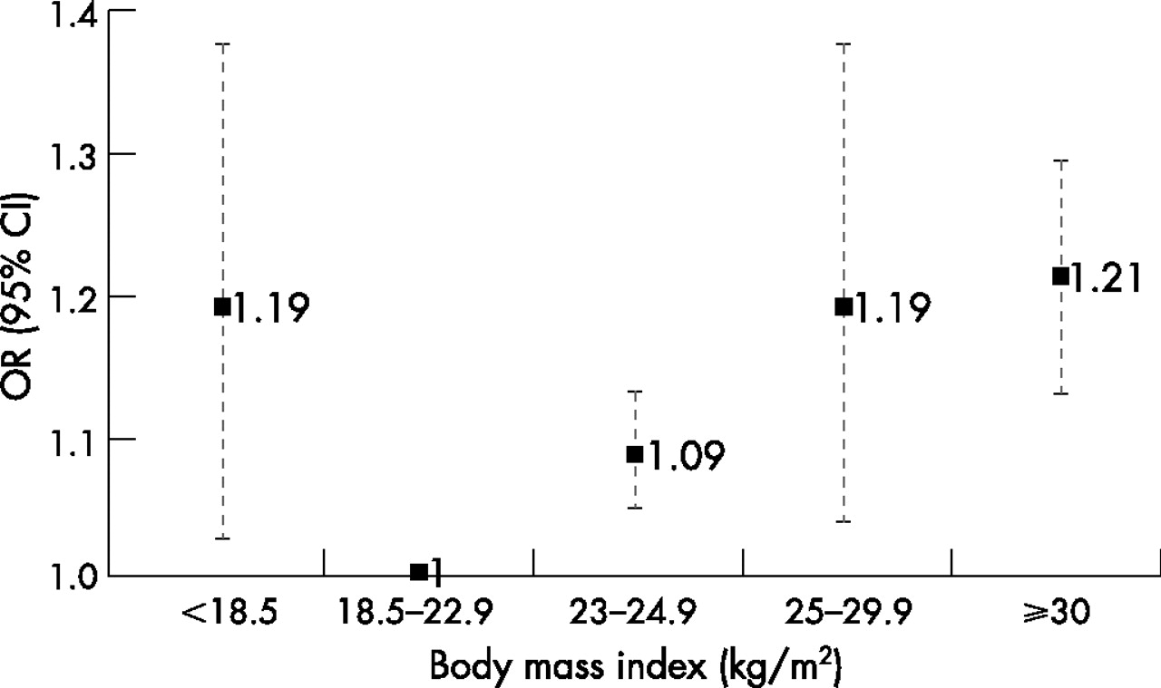
Table 3 presents the mutually adjusted odds ratios (ORs) and the 95% confidence intervals (CIs) for the risk of being underweight, pre-overweight, overweight and obese for the exposure variable and the covariates, using the normal BMI category as the reference. State-level income inequality was strongly associated with the levels of BMI (p<0.0001), even after controlling for a range of individual and state-level covariates. As shown in Figure 1, a one-standard deviation increase in Gini coefficient (which corresponds to approximately a 3% change in the Gini coefficient) increased the OR for being underweight by 1.19 (95% CI 1.03 to 1.37). The risk of being obese also increased by 21% (95% CI 1.13 to 1.29) for a one-standard deviation change in the Gini coefficient. The effect of Gini coefficient on the risk of being overweight was similar to that for obesity (OR 1.19, 95% CI 1.04 to 1.37). The Gini coefficient was also positively associated with the risk of being pre-overweight (OR 1.09, 95% CI 1.05 to 1.13). When we considered PCSDP as a control variable, instead of PCCE, the results were largely similar: a one-standard deviation increase in Gini coefficient increased the odds ratio for being underweight by 1.19 (95% CI 1.02 to 1.39). The OR of being obese increased by 10% (95% CI 1.04 to 1.18) for a one-standard deviation increase in the Gini coefficient. The effect of Gini coefficient on the risk of being overweight was similar to that for obesity, except that the estimate had lower statistical precision. The Gini coefficient was also positively associated with the risk of being pre-overweight.

We conducted additional tests of interaction (not reported) between state Gini coefficient and women’s standard of living index to verify if the effect of state Gini coefficient was confined to specific socioeconomic groups, but we did not find support for this hypothesis. We also considered models in which the state Gini coefficient measured in 1993–94 was used and obtained results similar to those reported here. Indeed, the correlation between state Gini coefficient in the two periods (1993–94 and 1999–00) was 0.78.

Other notable results included the strong positive association between state per capita consumption expenditure and risk of being pre-overweight (OR 1.12, 95% 1.09 to 1.16), overweight (OR 1.18, 95% 1.02 to 1.36) and obese (OR 1.24, 95% 1.19 to 1.30), with the ORs expressing one standard deviation increase in state per capita consumption expenditure (Table 3). However, increases in state per capita consumption expenditure did not substantially decrease the risk of being underweight and the relationship was statistically insignificant (OR 0.96, 95% CI 0.83 to 1.13). These associations were largely similar when we considered state average per capita net state domestic product. At the individual level, socioeconomic position was a strong predictor of body mass index: on average, higher levels of education or standard of living decreased the risk of being undernourished and increased the risk of being overnourished (Table 3).

DISCUSSION

This analysis found an association between state income inequality and levels of nutritional status, as measured by BMI, even after adjusting for a range of individual and state-level covariates in India. The adverse contextual effect of state income inequality is observed for the risk of being underweight as well as for each of the categories that characterise overnutrition (i.e. pre-overweight, overweight and obese). It is important to emphasise that what we report is a contextual effect of income inequality, after adjusting for individual-level factors, including economic standard of living, which we know has a clear relationship to nutritional status (in that women of low socioeconomic status experience the greatest risk for underweight and those in high socioeconomic status experience the greatest risk for being pre-overweight, overweight and obese)^6,42–44, a pattern also observed in this study. Thus, the context of inequality seems to accentuate the income-based disparities in consumption (reflected in people’s BMI).

Why should income inequality be adversely associated with both undernutrition and overnutrition? An insightful analogy can be drawn with the causes of famines. Famines, as we now understand, are caused not so much by a shortage of food as by the maldistribution of food.⁴⁵ In a similar manner, the simultaneous presence of under- and overnutrition probably reflects the maldistribution of resources in food and as well other domains of critical importance to nutritional status. Thus, highly unequal states are characterised by the simultaneous existence of overconsumption by privileged groups and food insecurity among the poor. In addition to being an indicator of maldistributed resources, income inequality may also be a marker of a less generous, or inefficient, public distribution system, e.g. as a result of corruption.⁷ For instance, it has been shown that the non-poor are more likely than the poor to use public systems designed to provide shelter, water, sanitation and sewerage, health care and food grains,⁴⁶ suggesting that public distribution systems in many communities are poorly designed to meet the needs of the poor, a necessary condition for overcoming the burden of undernutrition. At the same time, it is likely that existing public distribution systems are vulnerable to manipulation by vested interests, a characteristic more likely to be present in states with high levels of income inequality and low social cohesion.

Indeed, there is evidence to suggest that one of the flagship programmes aimed at improving nutrition of children and mothers – the Integrated Child Development Scheme (ICDS) – is regressive in several ways.⁴⁷ First, coverage of the programme is highest in states with the lowest levels of undernutrition. Second, coverage of the ICDS programme tends to be higher in states with high economic growth. Finally, in the poorer states, government budgetary allocations for the ICDS programme per undernourished child is lower. Indeed, poorer states also tend to spend only 65–75% of their allocation, suggesting poor governance. The regressive nature of this programme increased in the 1990s.⁴⁷ Thus, it is possible that there may be other contextual features of high-inequality states that make the goal of eliminating undernutrition difficult.

The fact that, on average, coverage of the ICDS programme tends to be greater in the richer states has led to the hypothesis that economic growth may eventually lead to a reduction in undernutrition through a trickle-down mechanism. However, in our analysis we could find only partial support for this. For instance, although women in richer states were more likely to be overnourished, there was no evidence that in these states the risk for underweight was actually lower than in states with considerably lower levels of economic growth. In a previous study, it was reported that for women in richer states the risk of being underweight increased for those in the lowest quintile of standard of living and decreased for those in the highest quintile.⁶ This again suggest that the health dividends of aggregate economic development seem to accrue largely to better-off sections of the population.

The following caveats should be borne in mind when considering our study findings. BMI was the only measure of nutritional status available. While a low level of BMI is likely to be a valid proxy for chronic energy deficiency in an individual, BMI does not adequately correlate with measures of body fat, which, for any value of BMI, may be higher in Indians than in other populations.^48,49 Thus, for any given BMI, the risk for the consequences of obesity, such as diabetes and cardiovascular disease, may be greater among Indians than in the populations on which BMI standards were initially developed.⁵⁰ These factors may limit the ability of our study to estimate the true burden of chronic diseases and mortality associated with undernutrition and overnutrition; however, in the Indian context, women’s BMI may have particular relevance because of its impact on the health of their offspring. Women of low pre-pregnancy BMI have lower-birthweight babies,⁵¹ and the evidence that low birthweight and low maternal BMI are associated with increased risk of adulthood chronic disease among offspring is consistent and universal.⁵² Indeed, the coexistence of undernutrition and overnutrition in India also means that the consequences of maternal obesity – high birthweight and a higher risk of diabetes among offspring – will increasingly be seen.⁵² As Osmani and Sen point out,²⁰ gender inequality can contribute to the intergenerational transmission of poor health through poor intrauterine and early life course exposures. It should also be noted that our findings relate to ever-married women between the ages of 15 and 49, even though it has the advantage of being nationally representative. However, the patterns observed in this study with regards to the relationship between nutritional status and individual covariates (including socioeconomic position) is consistent with prior studies on women and men,^42–44 thus strengthening the general relevance of our findings.

In conclusion, our study has shown an association between state income inequality and the concurrent presence of risk of individual underweight and overweight. Focusing on overall economic equity – especially during phases of health and economic transition – is likely to address this dual burden.